A spatial and temporal analysis of Australian climate fields

A Spatial and Temporal Analysis of

Australian Climate Fields

Jennifer L. Kesteven

Centre for Resource and Environmental Studies

November, 1998

Declaration

This thesis represents independent and original research except as indicated below and in the acknowledgements.

The ANUSPLIN suite of programs was written by Dr. Hutchinson and the brief descriptions in Appendix B are from the programs’ documentation. The Australian DEM and coastline were also provided by Dr. Hutchinson.

The circular GIF viewer program was written by Jim Throssell and developed in conjunction with him.

A very brief presentation of the data homogeneity and a short description of the space time models were presented in a paper given at the International Geographic Systems and environmental modelling conference held in Santa Fe, New Mexico, January

1996.

Parts of the section on the Australian climate and some of the maps were used in: Laughlin G. 1997. The user's guide to the Australia coast, New Holland, Sydney.

The surfaces were briefly described and proposed in:

Larson J.W., Taylor J.A., Kesteven J.L, Hutchinson M.F, Bates G.T. and Oglesby R.J. 1994. Regional-scale climate studies of Australia using RegCM2, a paper presented to the International Congress on Modelling and Simulation, Newcastle, November 27-30, 1995.

A variation of the music files was exhibited at the Canberra School of Art, 18-29 August 1997 in "Monga, An Exhibition of Field Work in Monga State Forest.

Acknowledgements

I would like to thank all my supervisors for their encouragement and the interest they have shown in this work.

I have been lucky to have had Michael Hutchinson as a supervisor, he has given freely of his time and invaluable advice. This thesis would not have been possible without him and his interpolation programs. He has been a great friend and the best of supervisors.

Janette Lindesay who joined the supervisory board at a difficult time and fitted in very easily. I would like to thank her for her climatological advice and her friendship. John Taylor, especially for his interest and encouragement to investigate. He also provided the bulk of the hardware used in the thesis and gave me an opportunity to run some global climate models.

I would like to thank Ken Johnston and Chris Trevitt all those cups of coffee and support in the early stages of my thesis.

There are many people at CRES I would like to thank for providing an interesting and stimulating environment within which this research was undertaken. Henry Nix, firstly, as director of CRES for making available the Centre’s resources, and for creating a great environment which is supportive and stimulating. Mark Greenaway for maintaining the computer system, which was essential for the successful output of the thesis, and with help when things go wrong. Rob McArthur provided help in the initial computer learning stage and set me onto the PERL programming language. I would like to thank all of the support staff. I would particularly like to thank Helen, John Mulquiney and John Gallant for the fun and the intellectual stimulus and George for the sustenance.

Jim Throssell for providing the circular viewer presented on the CD-ROM, and for his thought-provoking visits.

Finally, I would like to thank my family and friends for their constant encouragement and support throughout this course of study

Abstract

This study is an exploration of the methods of spatial and temporal analysis and extension, focused on an investigation of Australian climate fields. The analysis is presented as a progression from the one-dimensional temporal analysis of site data, to the investigation of the spline spatial interpolation method, to higher dimensional spatio-temporal modelling. This study also forms the foundation for further spatio- temporal modelling of other variables, particularly rainfall.

Table of Contents

Declaration

Acknowledgements

Abstract

List of Tables

List of Figures

List of abbreviations and acronyms used

List of Chapter Title Page Images

Chapter 1. An Analytical Framework for the Spatial and

Temporal Extension of Climate Site Data

1

Introduction 2

Overview 3

The Australian climate 6

The general circulation in the Australian region 7 Surface pressure patterns and wind in the Australasian region 9 Temperatures on the Australian continent 11

Rainfall 11

Space and time scales 13

Methodology 16

Conclusions 17

Chapter 2. The Spatio-temporal Station Climate Database

Introduction 21

The climatological elements and their measurement 21

Pressure 22

Temperature 22

Precipitation 23

Lapse rates 24

Climatological data 25

The pressure and temperature data set 26

The Bureau of Meteorology three-hourly records 26

Data set homogeneity 27

The derived data sets 28

Station data network 32

Temporal coverage 32

Spatial coverage 33

Topographic coverage 33

The Bureau of Meteorology monthly rainfall records 34

Rainfall percentiles/deciles 35

Conclusions 37

Chapter 3. The Spatial Interpolation of Climatic Variables.

Introduction 40

Established methods of statistical interpolation 40

Local interpolation methods 41

Moving average methods 41

Kriging 42

Thin plate smoothing splines 42

Partial thin plate smoothing splines 44

Errors in the model 46

Advantages of thin plate smoothing splines 47

The ANUSPLIN computer package 48

Fitting surfaces with SPLINA and SPLINB 49

Input data and options 51

Output statistics 52

Output fdes 56

From surface coefficient files to maps 57

ANUSPLIN assessment 57

Determination of the choice of various SPLINA and SPLINB input

options 57

Visual assessment 59

Daily pressure 59

Bureau of Meteorology rainfall maps 60

Actual versus interpolated values 62

Conclusions 63

Chapter 4. Fitting the Australian Climate Surfaces

Introduction 66

The monthly pressure and temperature surfaces 67

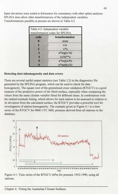
The monthly pressure and temperature surface construction 67 Detecting data inhomogeneity and data errors 68 Estimating true station or barometer elevation using SPLINA 73

Adequacy of the number of stations 74

Errors 75

Environmental lapse rates 79

The monthly long term average surfaces 82

Weighting by local variance estimates 82

Weighting by length of record 84

Uniform weighting 84

Equal weighting with SPLINB 86

vii

Surface long term averages 88

Fitting the rainfall percentile surfaces 88

Conclusions

90

Chapter 5. The Australian Spatio-temporal Climate Database

and Mapping Techniques Used to Describe the Database

Introduction

94

The ‘primitive’ surfaces

95

The derived surfaces

98

Logical models for specific times

99

Data extraction using DEMs

99

Aspect and slope maps

100

Temperature difference surfaces 102

Logical models representing change over time

103

Anomalies

103

Monthly lag surfaces

104

Diurnal difference surfaces

105

Spatio-temporal databases

106

Mapping techniques used to describe the spatio-temporal database

107

Graphs showing long term averages or trends in the data set

108

The long term Australian monthly average temperature and

pressure values

108

Previous studies of trends in temperature and pressure over

Australia

109

Trends in the spatial temperature and pressure data sets

1

0

Previous studies of trends in rainfall over Australia

114

Trends in the rainfall percentiles 114

Map images 11

5

Snapshots and composite images

116

Animation 11

7

Sound

119

The sound sequences

121

Combining sound and animation

123

Conclusions

123

Chapter 6. The spatial Models

125

Introduction

126

The spatial statistical models

127

Estimating the dew-point temperature

128

The spatial regression dew point temperature models

129

Incorporating dependencies of climatic variables on large scale synoptic

features

135

Rainfall models

137

Incorporating dependencies of rainfall on synoptic patterns 139

Spatial statistical forecasting 142

Climate prediction in Australia 142

Spatial lag linear regression model 142

Conclusions 147

Chapter 7. The Spatio-temporal Spline Models

Introduction 150

Implementation Issues for the space-time spline model 151

Computation issues 151

Space-time issues 152

The 'absolute' time spline Model 1 153

The event 'time' spline Model 2 157

Model 2 A - 'event' time as a mapping of the long term average values 157 Model 2B - 'event' time as a mapping of the local long term average

values 161

Determining the Model input options 162

The partial spline Models 163

The spline Models 165

Selecting the pseudo-time scale by hindcasting 167

Comparison of the output from the lag regression model and the

space-time spline models 169

Conclusions 173

Chapter 8 - Summary of Findings and Conclusions, Including

Research Directions and Potential Applications of

Methodology.

Introduction 176

Summary of findings and conclusions 176

The production of a temporally homogeneous station climate database 177 An assessment of the appropriateness of the spline interpolation method

for the spatial extension of climatic variables 177 The development of a monthly 'primitive' surfaces for Australian climate 178 The production of gridded estimates of derived climatic variables by

applying logical models to the primary climate variables. 179 The investigation of the points of a 2.5 x 2.5 degree grid of estimates of

climatic variables for an assessment of climate variability and change 179 The investigation of mapping techniques for displaying the spatio-

temporal database 180

The spatial interpolation of the correlation parameters and the regression

models 180

The production of the dew-point temperature space-time spline model 181

Future research directions 182

Interpolation issues 182

Climate Change and variability 183

The application of advanced graphical techniques 183

Climatic Models 184

Space-time spline model 184

Potential applications of methodology to climatological and

environmental issues 185

Climate Impact Assessment 186

Long term climatic predictions 186

Conservation of climatically sensitive environmental regions 186

Conclusions 187

Bibliography

Appendix A: The accompanying computer disk.

201

Appendix B: The ANUSPLIN Programs.

202

Appendix C: List of stations used in the pressure and

List of Tables

Table 3.1 Input options and description for SPLINA and SPLINB. 51 Table 3.2a Summary statistics from the diagnostics file, all stations,

pressure, July 1974. All statistics except error and signal in hPa. 54 Table 3.2b Explanation of summary statistics. 54 Table 3.3 Highest ten ranked root mean square residuals (from stations),

all stations, pressure, July 1974. 55 Table 3.4 List of the data and fitted values and standard errors for the first

and last three stations in the data file, all stations, pressure, July

1974. 55

Table 3.5 Output files from SPLINA and SPLINB. 56 Table 3.6 RTGCV for January 1952, 1968 and 1989 pressure surfaces for

both the spline and partial spline models, for various scales of

elevation. 58

Table 3.7 RTGCV for January 1952, 1968 and 1989 pressure surfaces for both the spline and partial spline models, for various order of

spline models. 59

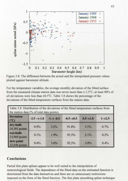
Table 3.8 Distribution of the deviations of the fitted temperature surfaces

from the station data (% of total data points). 63 Table 4.1 The input options that were used for SPLINA to produce the

pressure surfaces. 67

Table 4.2 Independent variable transformation codes for SPLINA. 68 Table 4.3 Ranked root mean square residuals (hPa) for pressure June

1952, December 1960 and January 1982. 69 Table 4.4 Ranked root mean square residuals (hPa) for pressure June

1952, December 1960 and January 1982 for surfaces created

with the reduced number of stations. 71 Table 4.5 Output statistics for the January 1989 pressure surface as

estimated from the 1989 equivalent of the January 1952 stations and as estimated from the full January 1989 data set. 75 Table 4.6 Output statistics for the January and July 1989 MSL pressure

and temperature surfaces. 79

Table 4.7a Output statistics for the January LTA MSL pressure surfaces

(all 125 stations using SPLINA). 83 Table 4.7b Output statistics for the July LTA MSL pressure surfaces (all

125 stations using SPLINA). 84

Table 4.8a The spline and partial spline SPLINB output statistics for the

January LTA MSL pressure surfaces. 86 Table 4.8b The spline and partial spline SPLINB output statistics for the

July LTA MSL pressure surfaces. 87

Table 5.1 The number of surfaces in the sets which make up the

Table 6.1 Percentage variance for the dew point regression models for

mid season months. 132

Table 6.2 Percentage variance for the dew point regression models as a function of the wet-bulb depression and pressure, for mid

season months. 135

Table 6.3 Percentage variance for the temperature regression models (as a

function of components of the pressure) for January and July. 137 Table 6.4 Percentage variance explained for rainfall percentile regression

models for mid-season months. 139

Table 6.5 Percentage variance for rainfall percentile regression models (as

a function of components of the pressure) for January and July. 140 Table 6.6 Percentage variance for the dew point lag regression models as

a function of lags 1, 2 and 3. 144 Table 7.1 The validation rms, maximum difference, error, signal and

RTGCV for the 'absolute' time dew-point temperature spline

Model 1 for April 1989. 155

Table 7.2 The average validation rms for the different scale options for the 'absolute' time dew-point temperature spline Model 1 for

1989 and 1990. 157

Table 7.3 The rms, maximum difference, RTGCV for the long-term average 'event' dew-point temperature spline Model 2A for

April 1989. 159

Table 7.4 The average validation rms for the different scale options for the event time dew-point temperature spline Model 2A for 1989

and 1990. 160

Table 7.5 The error, signal, RTGCV, validation rms, maximum difference for the full spline Dew Point temperature Model 2B for April

1989. 162

Table 7.6 The error, signal, RTGCV, validation rms, maximum difference

for the partial spline Model 2B, for April 1989. 164 Table 7.7 The average validation rms for the different scale options for

the 'event' time dew-point temperature spline Model 2B for

1989 and 1990. 168

Table 7.8 The average validation rms for the long-term average, the lag regression model and the spatio-temporal spline models for

List of Figures

Figure 1.1 Map showing the topography and feature names (source:

Hammond World Atlas). 6 Figure 1.2 The Intertropical Convergence Zone (ITCZ) over SE Asia and

Australia in July and January (source: Crowder 1995). 7 Figure 1.3 Air masses of Australia (source: Johnson 1992). 9 Figure 1.4 Mean pressure in January and July, 0900 local standard time

(LST) (adapted from Gentilli 1971). 10 Figure 1.5 Australian January maximum and July minimum air

temperatures over Australia (source: Johnson 1992). 11 Figure 1.6 Median monthly rainfall for January and July (source:

Crowder 1995). 12 Figure 1.7 Characteristic time and space scales, with associated

atmospheric phenomena (source: Sturman and Tapper 1996). 14 Figure 2.1 Canberra 0800 and 0900 LST, 1970 -1990, and Canberra 1100

and 1200 LST, 1970-1990. 29 Figure 2.2 Actual and interpolated pressure and temperature values for

Alice Springs for the 15th of July 1969 and 1989. 30 Figure 2.3 Stations with complete records, 1952-1990. 31 Figure 2.4 Number of stations used per year. 32 Figure 2.5 Station distributions for January 1952, 1982 and 1989. 33 Figure 2.6 Station DEMs for 1952, 1982 and 1989, and Australian 0.1°

DEM. 34 Figure 2.7 Locations of the 3160 Bureau of Meteorology stations with

continuous monthly rainfall data, 1952-1990. 35 Figure 2.8 Monthly rainfall totals versus monthly rainfall percentiles at

Perth, Darwin, Alice Springs and Canberra for January and July

from 1952 to 1990. 37 Figure 3.1 From data files to maps using the ANUSPLIN computer

package. 49 Figure 3.2 Flowchart of the SPLINA fitting approach. 50 Figure 3.3 GCV versus log RHO for pressure, January 1988. 56 Figure 3.4 MSL pressure maps for 15 January 1968 from (a) BoM

hand-drawn and (b) SPLINA. 60 Figure 3.5 The location of the stations coloured in the decile values for

the summer of 1993/4. 61 Figure 3.6 Decile values for the summer of 1993/4 (a) BoM manually

analysed maps based on district averages and selected stations derived from telegraphic reports, (source: BoM); (b) MAPGEN GIS package output, (source: BoM); (c) ANUSPLIN package output, and (d) ARCINFO GIS package

Figure 3.7 The actual station pressure values plotted against interpolated

values. 62 Figure 3.8 The difference between the actual and the interpolated

pressure values plotted against barometer altitude. 63 Figure 4.1 Time series of the RTGCV (hPa) for pressure 1952-1990,

using all stations. 68 Figure 4.2 Stations with high root mean square residuals for 0000 UTC

pressure 1952-1990. 70 Figure 4.3 Time series of the RTGCV in hPa for pressure 1952-1990, for

the reduced data set. 71 Figure 4.4 Time series of the RTGCV in hPa for pressure 1952-1990, for

the final data set used to produce the surfaces. 72 Figure 4.5 Examples of pressure and temperature surfaces. 73 Figure 4.6 Location of stations in the January 1952 (a) and 1989 (b) data

sets, and the January 1989 pressure surface as estimated from the equivalent of the January 1952 stations (c) and from the

full January 1989 data set (d). 74 Figure 4.7 Estimated standard prediction errors for January 1989 and

1982 pressure surfaces and the extraction grids used. 77 Figure 4.8 Estimated prediction errors for January and July 1989 MSL

pressure, dry-bulb, wet-bulb and dew-point temperatures. 78 Figure 4.9 Long term Environmental Lapse Rates (ELR). 80 Figure 4.10 Monthly fitted environmental lapse rates. 81 Figure 4.11 The maps produced from the different SPLINA weighting

methods for the January and July long-term pressure averages. 85 Figure 4.12 The spline and partial spline SPLINB surfaces for the January

and July long term averages. 87 Figure 4.13 Surface long term averages (SFLTA) for mid season months. 88 Figure 4.14 Maps of monthly percentiles across Australia from May to

August for 1973 and 1982. 90 Figure 5.1 July MSL pressure, rainfall deciles and the MSL dew-point

temperature for 1977 to 1980. 97 Figure 5.2 January and July SFLTA MSL dry-bulb temperature surfaces

for 0000, 0300, 0600 and 0900 UTC. 98 Figure 5.3 January and July 1989 MSL temperature surfaces used in

combination with the Australian DEM to give the surface

values. 99 Figure 5.4 MSL pressure average, aspect and slope maps for January and

July 1989. 100 Figure 5.5 MSL dry-bulb temperature average, aspect and slope maps for

Figure 5.9 Figure 5.10 Figure 5.11 Figure 5.12 Figure 5.13 Figure 5.14 Figure 5.15 Figure 5.16 Figure 5.17 Figure 5.18 Figure 5.19 Figure 6.1 Figure 6.2 Figure 6.3 Figure 6.4 Figure 6.5 Figure 6.6 Figure 6.7 Figure 6.8 Figure 6.9 Figure 7.1 Figure 7.2

Diurnal range for MSL dry-bulb temperature surfaces for January and July 1989. Australian MSL average SFLTA pressure and temperature. 120 month (10 year) moving average of the Australian MSL average for temperature and pressure, 1952-1990. 10° grid point 120 month (10 year) moving average for pressure and temperature (dry-bulb, wet-bulb, wet-bulb depression, and dew-point), 1952-1990. 120 month moving average wet bulb depression versus the 120 month moving average dew point temperature average

1952 to 1990. 120 month moving average of monthly rainfall percentiles for

Australia and the SOI from January 1952 to December 1990. 120 month moving average of monthly rainfall percentiles for Australian 10° grid points from January 1952 to December

1990. A composite image of the July LTA and all monthly AVG

MSL Pressure snapshots 1952-1990. The Cyclic GIF viewer. The dry- and wet-bulb temperature anomalies January 1952 to

December 1990. The converted musical notation for dry- and wet-bulb for January 1952 to December 1954. Average monthly Td values and the values estimated from T and Tw using psychometric tables for selected stations for

1989. The 119 Australian 2.5° by 2.5° grid points.

The MSL dew-point regression model A. The MSL dew point regression model B. The output from the dew-point temperature interpolation, the dew-point regression models A and B, and the Linacre model (ELRI) for mid-season months in 1989 and 1990.

The dew-point lag regression model. The validation rms for the lag regression B models 1989 and

1990. The validation rms and the anomaly rms for all months 1989 and 1990. The long-term surface average, the interpolated average surface and the output from the lag model B for all months for

both 1989 and 1990. The monthly average dew-point temperature and monthly anomaly dew-point temperature surfaces for January to April

1989. A conceptual spline spatio-temporal dew point temperature

using monthly values for January to April 1989. 105 108

1 1 1

Figure 7.3 The 'absolute' time spline dew point temperature anomaly

Model 1 for January to April 1989. 155 Figure 7.4 The output grids for the spline Model 1 for different time

dimension scale options. 156 Figure 7.5 The validation rms for all months from January 1989 to

December 1990 for the different scales fitted. 156 Figure 7.6 The average Australian SFLTA dew point temperatures. 158 Figure 7.7 The 'event' time spline dew point temperature Model 2A for

January to April 1989. 158 Figure 7.8 The output grids for the spline Model 2A for different time

dimension scale options. 159 Figure 7.9 The Model 2 validation rms for all months from January 1989

to December 1990 for the different scales fitted. 160 Figure 7.10 The long term average dew-point temperature transects

through 20°S and 30°S. 161 Figure 7.11 Varying scale and order space-time spline Model 2B outputs

for April 1989. 163 Figure 7.12 Outputs for varying order and number of covariates for the

space-time partial spline Model 2B, for January to April 1989. 165 Figure 7.13 The validation rms for the spline Model 2B. 166 Figure 7.14 The output for the different scaling options from the second

order spline Model 2B for mid-season months for 1989 and

1990. 167 Figure 7.15 The minimum validation rms and the validation rms as

selected by the hindcast model. 168 Figure 7.16 The anomaly rms, the validation rms from the lag regression

Model and the 'best' validation rms for the forecast spline

Model 1, 2A and 2B. 170 Figure 7.17 The anomaly rms, the validation rms from the lag regression

Model and the validation rms for the season scale Model 1, the fixed i* 15 scale Model 2A and hindcast scale Model 2B. 170 Figure 7.18 The monthly average dew-point temperature ('primitive'), the

output from the dew-point temperature lag regression model and the output for the spatio-temporal spline models for 1989. 171 Figure 7.19 The monthly average dew-point temperature ('primitive'), the

List of abbreviations and acronyms used

A C T A u s tra lia n C a p ita l T e rrito ry A V G m o n th ly av e ra g e

B o M B u re a u o f M e te o ro lo g y °C d e g re e s C e lsiu s

C D c o m p u te r d isk

D A L R d ry a d ia b a tic la p se ra te D E M D ig ita l E le v a tio n M o d e l D S T d a y lig h t sa v in g tim e E L R e n v iro n m e n ta l la p s e ra te E N S O E l N in o S o u th e rn O s c illa tio n

E R IN E n v iro n m e n t R e s o u rc e In fo rm a tio n N e tw o rk G C M G lo b a l C lim a te M o d e l

G C V g e n e ra lis e d cro ss v a lid a tio n G IS G e o g ra p h ic In fo rm a tio n S y ste m h P a h e c to p a s c a ls

IT C Z In te rtro p ic a l C o n v e rg e n c e Z o n e

K K e lv in

k m k ilo m e tre

L S T lo c a l sta n d a rd tim e

L T A L o n g -te rm m o n th ly a v e ra g e s

M ID I M u sic a l In s tru m e n t D ig ita l In te rfa c e

m m m illim e tre

M S E m e a n s q u a re e rro r M S L m e a n se a -le v e l M S R m e a n s q u a re re s id u a l R H O s m o o th in g p a ra m e te r

rm s ro o t m e a n sq u a re (re s id u a ls )

R T G C V sq u a re ro o t o f th e g e n e ra lis e d c ro s s v a lid a tio n R T M S E s q u a re ro o t o f th e m e a n s q u a re e rro r

R T M S R s q u a re ro o t o f th e m e a n sq u a re re s id u a l R T V A R s q u a re ro o t o f th e e rro r v a ria n c e e s tim a te S A L R s a tu ra te d a d ia b a tic la p s e ra te

S F L T A s u rfa c e lo n g te rm a v e ra g e S O I S o u th e rn O s c illa tio n In d e x S S T s e a s u rfa c e te m p e ra tu re

T d ry -b u lb te m p e ra tu re

Td D e w -p o in t te m p e ra tu re

Tmin m in im u m te m p e ra tu re

T M S E tru e m e a n s q u a re e rro r

T w w e t-b u lb te m p e ra tu re

Chapter Title Page Images

T

Chapter 1: Rainbow, near Braidwood, NSW

Chapter 2: Dawn, Meringo, NSW

Chapter 3: Fresh snow fall, Little Thredbo Homestead, NSW

Chapter 4: Thredbo, NSW

Chapter 5: Storm, South Coast, NSW

Chapter 6: Storm, Canberra, ACT

Chapter 7: Sunset, Lismore, NSW

Chapter 1. An Analytical Framework

for the Spatial and Temporal Extension

Introduction

Climate plays a crucial role in determining earth surface processes. It exerts fundamental controls on the distribution of natural vegetation, on soils and on the activities of people. As the world’s population increases, the demand for food, water and energy steadily increases, while the ability to meet those needs will remain subject to the vagaries of climate. The world is becoming increasingly dependent on the stability of the present seemingly ‘normal’ climate as it approaches full utilization of the water, land and air which supply the food and receive the wastes. Managing this climate dependency requires coordinated management of the world’s resources and a thorough knowledge of the behaviour of climate.

Climate reflects the long-term patterns of weather and thus meteorological

observations are fundamental to the development of an understanding of climate and climate change. It is essential that the relevant data be collected on a long-term basis in order to acquire the necessary statistics of climate. Due to the need for improved weather forecasts, the Australian network of meteorological observation stations has grown extensively since the production of the first weather map in 1877 (Colls and Whitaker 1990). Thousands of pieces of meteorological data are collected around Australia on a daily basis; however, they are not available for all times for every location across the continent. These data, then, must be extended in both space and time to adequately document the climatic events that have occurred in the past, and to monitor the climate processes presently occurring.

This study is an exploration of the methods of spatial and temporal analysis and extension, focused on an investigation of Australian climate fields. The analysis is presented as a progression from the one-dimensional temporal analysis of site data, to the investigation of the thin plate smoothing spline spatial interpolation method, to higher dimensional spatio-temporal modelling. This study also forms the foundation for further spatio-temporal modelling of other variables, particularly rainfall.

The broad objectives of the study are:

♦ the investigation of the characteristics of point data;

♦ the development of an Australian station climate database developed for specific UTC times;

♦ the extension of the station climate so that it is spatially and temporally complete; ♦ to contribute to the development of techniques for using the thin plate smoothing spline for the spatial extension, interpolation and prediction of climatic variables;

♦ the investigation of mapping techniques used to describe spatio-temporal databases and an assessment of climatic variability and change;

♦ the spatial-temporal prediction, by integration of the spatial and temporal

dimensions, of the climatic variables. This involves the development of a space-time model which deals with the space and time dimensions simultaneously.

The management and manipulation of megabytes of data have been essential to this study. Computer-based methods facilitate data analysis and spatial extension, and provide images which can enhance our capacity to view and interpret the climate information. Given the importance of high quality, spatially homogeneous data to the study of climatic variation and climate change, the work reported in this thesis aims to provide a spatially homogeneous Australian climatic database and to examine the temporal variability in that database. The climatic database developed here contains more than 20,000 graphics, animations of all the spatial time series, and the

continental anomaly time series transformed and presented as an audible signal which can be heard in conjunction with the animated time series. Due to the

practicalities of producing a thesis it is not possible to include these in the hard copy. There is, however, a computer disk (CD) attached to the thesis which includes the climatic database described here (see Appendix A). The CD also includes a version of the thesis which is linked interactively to the graphics. The use of the CD version is encouraged as it provides additional dimensions (visual and aural) to the material documented in the thesis.

Overview

All data have locations in time and space. Sometimes, when doing analysis on these data, it is necessary to take these locations explicitly into account. In few subjects can this be more true than in meteorology and climatology, as most variables in the atmospheric sciences can be viewed as spatio-temporal processes (e.g. sets of pressure and temperature measurements from a number of sites over a period of time). Space-time statistical models are an attempt to extend the historical data in time, and to interpolate across space. Estimation of climatic variables at unsampled times or unsampled spatial locations requires the extension of existing interpolation techniques into the space-time domain. The problem is simplified if the time

component is integrated out; the study then is reduced to the problem of interpolation and prediction in space only. Similarly the spatial dependence can be removed, allowing the application of time series methods.

As Ripley (1984) points out, advances in data logging are revolutionising not only areas of the natural sciences such as meteorology, but also the statistical methods which serve them. Meteorologists have available, particularly in recent years, volumes of data which are truly enormous in comparison with many other areas in which statistical methods are applied. Data are routinely collected on temperature, pressure, humidity and precipitation, wind, and other weather conditions. These data are collected by a variety of fixed or transient systems, including weather stations, ships, aircraft, buoys, balloons, radar and, most recently, satellites.

In developing methods for the spatial and temporal determination of climatic

variables, this study recognises the importance of the availability of data stations with sufficiently long records so that spatial interpolation errors are not large. The range of data available directly affects the choice of spatial and temporal scales. The ground- based network is the only source of daily surface weather data with extensive temporal coverage and near-complete continental land coverage. This data set, however, contains both spatial and temporal discontinuities which are discussed in Chapters 2 and 3.

It has been suggested that monthly space-time models, which may be reasonably well determined from standard meteorological networks, are sufficient to resolve much ecological and hydrological behaviour, at relatively fine spatial resolutions of a few kilometres (Hutchinson 1995a and 1995b). To achieve the objectives of the present study an integrated analysis of monthly pressure and temperature fields across Australia from January 1952 to December 1990 has been undertaken.

Weather is the state of the atmosphere at a particular point in time over a given region, while climate is a synthesis or generalisation of the weather observed over a longer time period. Meteorology and climatology represent the study of weather and climate respectively(Sturman and Tapper 1996). The different time scales have given rise to different methods used for spatial and temporal extension of the data. One method of spatial extension of meteorological data is to use purely subjective techniques. This method is still used by many practicing meteorologists, especially for pressure data. The data are reduced to mean sea-level (MSL) values at the station by local table calculation and contours are drawn by hand to represent the MSL pressure field. Daily pressure maps are still drawn in this way and produced

alongside computer generated maps. More recently, weather radar has been used to present three-dimensional cross-sections of storms, and remotely sensed data from satellites are used to map cloud patterns and cloud-top temperatures. Satellite data will become increasingly valuable as new methods of storing and analyzing large volumes of data are developed.

Studies of space-time variation in atmospheric science overlap with research in hydrology and ecology. They cover a wide range, both methodologically and in the nature of the problems investigated. Many studies in spatio-temporal modelling have concentrated on the spatial domain, by treating the time replications effectively as independent. Others have concentrated on the time domain, by ignoring the spatial interactions.

Neither the exclusively temporal nor the spatial approach are entirely satisfactory. Geostatistics offers a variety of methods to model data processes as realisations of random functions. These procedures have been applied primarily to spatial data. Applying such space-orientated approaches to spatio-temporal processes, however, may lead to the loss of valuable information in the time dimension.

Although apparently straightforward, this solution presents both theoretical and practical problems as there are major differences between temporal and spatial phenomena. Rouhani and Myers (1990) and Rouhani and Wackemagel (1990) suggest that these practical and theoretical problems are as follows:

1) One-dimensional temporal data are ordered, a characteristic not usually found in two- or three-dimensional spatial data, which do not exhibit such order as past, present and future. Also, space and time are measured on two different scales which cannot be compared in a physical sense.

2) The spatial locations available are often sparsely distributed, whereas the time series associated with each location are relatively long. The accuracies of estimated temporal and spatial structures are likely to be quite different.

3) Space-time data can often exhibit temporal periodicity and spatial non- stationarity. A variety of temporal periodicities have been observed, such as periodic seasonal cycles, pseudo-periodic climatic cycles, and non-periodic long term trends. The periodic component can be approached as a part of the trend, or the series can be treated as stationary. The spatial non-stationarity may be ignored in some cases; in others, however, it raises serious doubts about the spatial homogeneity assumption. In response to these problems, a new approach to the modelling of spatio-temporal data is proposed here. The differences in scale between the spatial and temporal data are discussed, and a method to overcome these differences, involving a combination of physical and statistical procedures, is presented. The method involves the

transformation of the time scale to a spatially distributed representation of the variable in question, in an attempt to deal with the apparent spatial non-stationarities and temporal periodicities in the meteorological data sets. This study proposes that the space-time covariance structure of climate can be used to develop a space-time model which incorporates time into the spline spatial model. This approach extends the existing spatial techniques by integrating the space and time domains. That is, the proposed solution is to consider the spatio-temporal phenomenon as a realisation of a spline function which incorporates one dimension for time with the remaining dimensions in space (usually two or three).

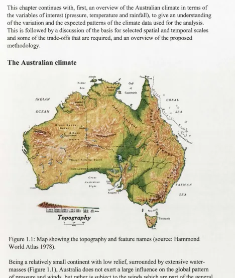
This chapter continues with, first, an overview of the Australian climate in terms of the variables of interest (pressure, temperature and rainfall), to give an understanding of the variation and the expected patterns of the climate data used for the analysis. This is followed by a discussion of the basis for selected spatial and temporal scales and some of the trade-offs that are required, and an overview of the proposed methodology.

The Australian climate

Topography

> Ü !

' S E A

T A S M A N

S E A

V i r CJ* 1 Tasmania

w

T i mo r S e a

I N D I A N

O C E A N

Figure 1.1: Map showing the topography and feature names (source: Hammond World Atlas 1978).

The general circulation in the Australian region

Australia spans latitudes from the tropics (10°S) to the lower middle latitudes (45°S) of the southern hemisphere. Much of the continent falls under the influence of the descending air and divergence which is characteristic of the belt of subtropical high pressure. In general this zone comprises vast areas of light winds and gently

subsiding air. Rain-bearing clouds are relatively few and the weather is usually fine. It is not surprising that the great deserts of the world are found in this zone.

In the winter months the subtropical high pressure belt is narrower than it is in summer and is broken into cells. The belt lies across the Australian continent around 29°S to 32°S, and a westerly wind regime covers the southern parts of the land mass where fronts embedded in this flow regularly bring periods of unsettled weather. To the south of the high pressure ridge a belt of low pressure characterised by strong westerly winds, can affect southern Australia and especially Tasmania. To the north fine weather prevails under the influence of the tropical easterlies.

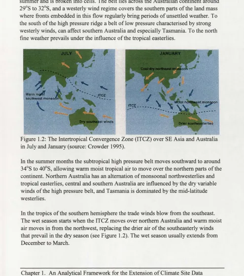
Figure 1.2: The Intertropical Convergence Zone (ITCZ) over SE Asia and Australia in July and January (source: Crowder 1995).

In the summer months the subtropical high pressure belt moves southward to around 34°S to 40°S, allowing warm moist tropical air to move over the northern parts of the continent. Northern Australia has an alternation of monsoonal northwesterlies and tropical easterlies, central and southern Australia are influenced by the dry variable winds of the high pressure belt, and Tasmania is dominated by the mid-latitude westerlies.

In the tropics of the southern hemisphere the trade winds blow from the southeast. The wet season starts when the ITCZ moves over northern Australia and warm moist air moves in from the northwest, replacing the drier air of the southeasterly winds that prevail in the dry season (see Figure 1.2). The wet season usually extends from December to March.

Between latitudes 40°S and 50°S is a zone of strong westerly winds, which develop in these latitudes as the oceans extend around the globe and winds are practically unimpeded by land. Southern Australia is usually on the northern margin of the westerlies and their influence is particularly noted in winter and spring when storms in the belt of extra-tropical cyclones are further north than usual. Western Tasmania is particularly affected by the westerlies which result in windy wet winters.

In the upper troposphere (around 200 hPa) the subtropical jet stream meanders over the continent throughout the year. There are intimate links between high-level flow and surface synoptic disturbances. The jet stream plays a role in creating and steering synoptic disturbances, and it contributes to the maintenance of the general circulation (Reiter 1961). In the Australian region the subtropical jet stream is more prominent than elsewhere, and is a feature over the continent for the entire year. Brook (1982) found the subtropical jet stream a consistent and persistent feature of the atmospheric circulation in the Australian region. Its existence is a direct result of the mechanism responsible for meridional transfer of heat.

There are marked seasonal variations in the subtropical jet stream. It is weaker in summer than in winter. There are also spatial changes in preferred jet-stream location both across the continent and between seasons (Gentilli 1971, Brook 1982). Both the seasonal and latitudinal features and the year to year variations of the jet stream are reflected in the behaviour of the depressions and anticyclones of the Australian region. The pressure trough between successive anticyclones is associated with an equatorward meander of the subtropical jet stream and its subsequent acceleration. Its main effect in winter is the formation of upper-air depressions. The magnitude and latitude of an anticyclone are also closely related to the speed and latitude of the subtropical jet stream (Reiter 1967, Gentilli 1971).

Significant deviations from the mean flow patterns occur as a function of longitude in both summer and winter. Apart from the major seasonal changes, some periods are found to be marked by strictly zonal flow with a single jet stream, while others have pronounced wave patterns or split jet configurations, with a single strong jet in the west and a double jet further east. The transition from the single to the double jet tends to occur at a preferred site for the formation of slow-moving intense ‘blocking’ anticyclones and of mid-tropospheric low-latitude depressions which play a large role in the rainfall regime of the Tasman Sea area (Brook 1982).

The southern hemisphere blocking systems are not well defined in monthly mean circulation fields, since they are generally less persistent or of smaller amplitude than in the northern hemisphere, due to the lack of major land masses in the southern mid­ latitude regions (Coughlan 1983). They are, nevertheless, sufficient to deflect

Winds in the middle troposphere (at the 500 hPa level) and above are the

counterparts of the surface winds, balancing equatorward surface flows by poleward winds, and vice versa. In the southern hemisphere the mean tropospheric flow departs little from a purely westerly direction, although there is a particularly strong westerly flow at 30°S to 45°S. The westerlies are stronger and more extensive in the southern than the northern hemisphere, due to fewer land obstructions. They are also stronger in winter than in summer as the temperature gradient between the equator and the poles increases. On any given day, however, the circulation pattem may display many small-scale weather disturbances travelling in an easterly direction.

Surface pressure patterns and wind in the Australasian region

As previously discussed, upper-level features play a major role in the creation and steering of the surface synoptic systems that produce the regional weather that is aggregated to provide the climate. Before looking at the role of these surface systems there is a need to understand that the origin of the air masses, which the surface pressure differences transport, which will have a predominant effect on the weather. Australia is affected by most of the major types of air masses: cold subpolar maritime air originating over the Southern Ocean, hot dry subtropical continental air

originating over the Australian continent, and warm moist Pacific and Indian subtropical maritime air originating over the Pacific and Indian oceans. Figure 1.3 shows that the air masses have different limits of penetration into the continent depending on the time of year (Johnson 1992).

The representation of the surface circulation for long periods (months, seasons, etc.) by charts of anticyclonicity and cyclonicity was developed during the early 1950s, to help solve the problem of extended long-range forecasting in Australia. Charts of seven-year averages (1946-1952) of monthly seasonal anticyclonicity and cyclonicity and their description were published by Karelsky (1954). Updated charts for the 15 years 1946-1960 were later published by Karelsky (1961) and also for the period

1952-1963 (Karelsky 1965). Charts of 23 year averages (1965-1987) of monthly anticyclonicity and cyclonicity have been published by Leighton and Deslandes (1991a, 1991b).

W in ter

Figure 1.3: Air masses of Australia (source: Johnson 1992).

At the surface the main atmospheric features of the Australian region which influence the weather are the high pressure systems or areas of divergence which tend to bring settled weather, especially to areas under the influence of the center of the system. Low pressure systems or areas of convergence to the south of the continent, with their associated fronts and relatively colder air masses, tend to bring most of south­ east Australia's winter weather.

Pressure (hPa)

1909 1919 1929 1939

Figure 1.4: Mean pressure in January and July, 0900 local standard time (LST) (adapted from Gentilli 1971).

In winter, the cooling of the land mass causes an increase in the density of the overlying air, and a consequent alteration in the barometric pattem. Figure 1.4 is adapted from Gentilli (1971) and shows the mean January and July surface pressure fields. The high-pressure belt moves northwards with the seasonal change, with a majority of the anticyclone tracks being between 29°S and 32°S (Karelsky 1954,

1961 and 1965, Gentilli 1971 and Streten 1982). There is, however, latitudinal variation; usually the track is at its furthest north over most of Australia in June-July, but, due to the greater lag in ocean temperatures off the east coast, the northward deflection can be retarded there until August-September.

During the winter the proximity of the mid-latitude depressions to the Australian mainland increases very rapidly to its July maximum (Karelsky 1965) with cyclonic centres passing near Tasmania. Any large depression well to the south of Australia produces a strong southerly flow, which may be as cold as 2°-3°C when it reaches the southern shore in winter.

systems moving north parallel to the east coast can result in gales and strong south­ easterly winds along the east coast.

Temperatures on the Australian continent

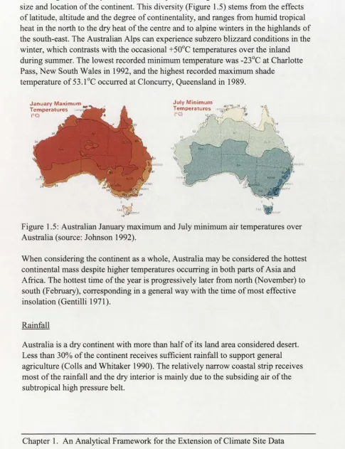
There is a great diversity of surface air temperature ranges across Australia due to the size and location of the continent. This diversity (Figure 1.5) stems from the effects of latitude, altitude and the degree of continentality, and ranges from humid tropical heat in the north to the dry heat of the centre and to alpine winters in the highlands of the south-east. The Australian Alps can experience subzero blizzard conditions in the winter, which contrasts with the occasional +50°C temperatures over the inland during summer. The lowest recorded minimum temperature was -23°C at Charlotte Pass, New South Wales in 1992, and the highest recorded maximum shade

temperature of 53.1°C occurred at Cloncurry, Queensland in 1989.

Figure 1.5: Australian January maximum and July minimum air temperatures over Australia (source: Johnson 1992).

When considering the continent as a whole, Australia may be considered the hottest continental mass despite higher temperatures occurring in both parts of Asia and Africa. The hottest time of the year is progressively later from north (November) to south (February), corresponding in a general way with the time of most effective insolation (Gentilli 1971).

Rainfall

Australia is a dry continent with more than half of its land area considered desert. Less than 30% of the continent receives sufficient rainfall to support general agriculture (Colls and Whitaker 1990). The relatively narrow coastal strip receives most of the rainfall and the dry interior is mainly due to the subsiding air of the subtropical high pressure belt.

When the subtropical high pressure belt moves northward in winter, dry southeasterly winds prevail over northern Australia, and southern Australia comes under the

influence of the winter westerlies. Cold fronts associated with depressions to the south of the continent move eastwards across southern Australia and are often accompanied by strong winds, heavy rain showers and snow in the alpine areas. Areas exposed to the westerlies, such as the southwest comer of Western Australia, southwestern Victoria, and particularly western Tasmania, have heavy winter

rainfalls, but most of the southeast part of the continent is more sheltered and rainfall more evenly distributed around the year.

Figure 1.6: Median monthly rainfall for January and July (source: Crowder 1995). When the subtropical high pressure belt moves over southern Australia in summer, the ITCZ and summer monsoon move in over northern Australia (see Figure 1.2). Moist northerly winds bring showers, thunderstorms and the threat of tropical cyclones to northern Australia.

Precipitation patterns are always complex in mountainous areas and their nature varying enormously from one mountainous region to another depending on the characteristics of the region (including height, orientation and location) and its interaction with the prevailing winds and storms that occur in the region. Australia is relatively flat and its mountains are small compared with those of all the other continents. Nevertheless, the Great Dividing Range and the escarpments which extend along the eastern seaboard, and the Alps of the southeast, are major factors in determining the climate of the continent and the distribution of water resources. The higher rainfall along the east coast of Australia is primarily due to the inflow of moist air from the ocean and the orographic influence of the Great Dividing Range. The heaviest rainfalls occur where moisture-laden winds are forced to flow up slopes of mountain ranges, and very arid areas can occur in the lee of mountains. The heaviest falls do not always occur at the tops of the highest mountains, as much of the

are the result of the southeast trade winds gathering moisture as they move over the Pacific Ocean and releasing large volumes of water as they strike the coast and move up the slopes of the ranges. Very heavy rainfalls also occur in winter in the

mountains of western Tasmania as this region is exposed to the westerlies.

Hutchinson and Bischof (1983) and Hutchinson (1995a) have shown the importance of incorporating vertically exaggerated topography in rainfall interpolation and analyses.

Space and time scales

The word ‘scale’ is used in many contexts and often connotes different aspects of space and time. Scale is the spatial or temporal dimension of an object or process. It should not be confused with cartographic scale which is the degree of spatial

reduction indicating the length used to represent a larger unit of measure. The monthly time scale and a spatial resolution of ten kilometres for the Australian continent have been selected as the temporal and spatial scales for this study.

Climates, ecosystems, and societies interact over a wide range of temporal and spatial scales. For temporal scales of a year or shorter, the space-time structure of

atmospheric phenomena has been reasonably well studied. There is a clear link between space and time scales and the nature of processes that dominate across the space and time spectrum (Orlanski 1975). These are summarised in Figure 1.7, which shows the range of scales and typical phenomena observed in the atmosphere. A consideration of the spatial scales of some important climatic phenomena suggests that a grid size on the order of 10 square kilometres and the use of the monthly time step would allow an adequate representation of key meso-scale processes that are related to synoptic scale meteorological events. Many other processes operate on finer spatial scales, but data limitations can preclude continental modelling at such scales.

The tremendous burden of sampling spatial variables adequately often means that existing data sources must be used. Sometimes available data determine research designs and space-time scales. This is especially true for broad-scale problems. Mathematical and statistical considerations may affect the selection of scales. Data handling thresholds are intertwined with time and space scales. This data-handling threshold has been moved to higher time-space resolution by technology. However, time and financial considerations constrain spatial scales, the number of variables considered and the time scales used.

Micro M<930 Macro --- 1--- (— .0 _{— 4—}a _—7 _{t--- 1}f>

a (J a --- 1---scale labels-after OrSanski (1975) VtMirn Mae tiis WiMiks Days Ifaurs Millies Second^

- M acro •

|~— Me>so— j

■ toe.it

- Micro •

Synoptic ~-|

y' Long waves

/'* Jet streams

Anlkrydoftes / / CydOlidS Hisnxuirw: Fronts /■/

/ Local winds Sguall lines

Th&irfcie«$S*ms y Lange ctamuws

Lee waves

/* Tornadoes , /

*' Sma* cunnAis

/

yt*

*“ Thermals Ousldevife Quldhg «ftee» Twtxjieflce finoghiiess Smalt-scale y

ir-ta mm ”1---1 km

l 1000 km

Characteristic horizontal distance scale

Scale labels,

after Oku

{1987}

Figure 1.7: Characteristic time and space scales, with associated atmospheric phenomena (source: Sturman and Tapper 1996).

The geographic literature is rich in philosophical discussions of spatial scales and methodological solutions for dealing with scale (e.g. Harvey 1969). There is, however, widespread agreement that, with changes in scale, different variables assume different degrees of importance. Moreover the value of a phenomenon at a particular place is usually dependent on causal processes operating at differing scales. The literature of the physical climatology of the earth’s surface also illustrates the pragmatic problem of matching time and space scales (Flohn 1981, Lewis 1995), as well as determining the nature of the variables which are important. The

methodological solutions already in existence need not be reinvented to more fully incorporate the spatial dimension in the modelling process and for the extension to broader scales of spatial analysis.

restricted to the size o f the phenomenon. It should be clear, however, that the addition o f the spatial dimension in the study o f nearly any process or phenomenon may involve a variety o f trade-offs. Models for broader-scale patterns result in reduced predictive accuracy at specific points or places, and the models are only as good as the finest resolution spatial data available.

Meentemeyer (1989) claims that researchers with similar propensities select similar scales and seem therefore to group together, and that perhaps this is caused by dominant paradigms, data sources, and other realities. Perhaps a better way to decide on proper scales is their efficacy in applications, that is not just studying weather and climate in isolation but applying it to modelling biodiversity or agricultural

distributions. Nevertheless it is worth noting Clark’s (1985) warning, that “no simple rules can automatically select the ‘proper’ scale for attention” .

A major constraint on the choice o f time step for this study was the computational requirements o f an analysis o f continental climate data. The spatial distribution o f monthly means can be reasonably determined from standard meteorological networks. Monthly surfaces and monthly mean surfaces have often been used in climatology (e.g. Allan and Haylock 1993, Kong 1995) and are used by the Bureau o f Meteorology as a method o f providing summary statistics (Bureau o f Meteorology

1968-1989). Atmospheric variables exhibit temporal variations consisting o f both regular periodic components and chaotic or random fluctuations. The former provide a good basis for prediction, while the latter cause real problems for both short- and long-term forecasting.

The monthly time scale incorporates much o f the spatial variability o f climate and is sufficient to resolve much o f the seasonal variation in ecological and hydrological activity and hence the spatial variability of dependent biological activity (Nix 1986,

Booth et al. 1987, Mackey et al. 1989 and Hutchinson et al. 1992). The BIOCLEM

program has successfully used the spatial distribution o f monthly mean climatic variables to predict the spatial distribution o f natural plant and animal species (Nix

1986). The monthly time scale has also been used as a basis for agro-climatic

classifications (Hutchinson et al. 1992).

Effective determination o f the spatial distribution o f mean climatic variables is also a necessary first step towards the development o f stochastic models o f the weather for more refined assessments o f the impacts o f climate (Hutchinson 1987, 1995b). This determination provides a basis for spatially interpolating and simulating actual

weather values at monthly, weekly and even daily time steps (Hungerford et a l 1989,

Hutchinson 1995b). The broader spatial scale o f monthly data also goes some way to meeting the broad spatial scales o f Global Climate Models (GCMs), and climatological

means play a crucial role in validating general circulation models (Gates et al. 1992).

While the monthly time step is appropriate for the assessment o f the Australian climate, it is important to note that there are limitations to the physical interpretability o f this

approach. As measurement time scales are lengthened, the estimate of variability of the phenomena is low because the monthly values vary less than the daily and/or hourly values upon which they are based. As the underlying processes tend to have shorter time scales, erroneous inferences about lower levels from the higher levels of aggregation can be made. For example, many factors are intricately related to the spatial distribution of surface air temperature on a local scale. Hourly air temperature distribution is directly influenced by factors such as solar radiation, precipitation, atmospheric movement on a larger scale, and various sizes of eddies. However, mean air temperature distributions during longer periods, such as the monthly mean, are mainly affected by the factors such as topography, vegetation and soil wetness. This is because spatial variations in the former factors are averaged over longer periods and thus their effects on spatial prediction of the mean air temperature disappear.

Methodology

The methodology applied in this study approaches the task of developing space-time climate models from standard meteorological networks in five steps.

The first step is to produce a standardised database appropriate for use in

interpolation of climatic variables on a continental scale. This includes obtaining data to provide an adequate sample of the spatial variation in the climatic variables of interest, and the determination of the criteria for station selection. The derivation of estimates for standard times is necessary for the removal of temporal discontinuities caused by the collection of data in different time zones, and to overcome

discontinuities in the climatic record as a result of the introduction of daylight saving time at some stations.

considered necessary to test the integrity of the spline function in producing the surfaces and to provide some useful insight into the interpolation of parameter surfaces. The procedure is based on regression techniques applied to spatial data and on the use of the thin plate splines to spatially extend parameter surfaces. These models, which attempt spatial-temporal prediction by applying regression and lag regression models to surface point data, and then spatially extending the model parameters. While these models were developed to test the integrity of the spline function in parameter surface construction, they also provide some useful models which can be used as a base against which the results from the next step can be compared.

The fifth step is the development of the space-time spline model, which models simultaneously the spatial and temporal anomaly correlations of climatic variables. The step is important, as the contemporaneous incorporation of time into the spatial model is not often done. The space-time spline model, while still under development, shows promise for modelling climatic variables at the monthly time scale. It also provides useful insights into the use of spline functions and has led to the formulation of a new approach to the integration of space and time scales.

The approach used in this investigation conveniently isolates different spatial and temporal aspects of climate model development. In particular it investigates the spatial and temporal dimensions separately before an attempt is made to integrate the dimensions. It identifies the climatic patterns existing over the Australian continent for the period from 1952 to 1990, and provides an insight into the spatio-temporal patterns and the modelling of these climatic variables.

Conclusions

This thesis applies the analytical framework as outlined above for the simultaneous spatial and temporal extension of climatic site data to develop models of particular variables and to support the future development of further models, including space- time models of rainfall. The eventual aim in the study is the incorporation of the space and time scales in a space-time spline cube. This work has involved a number of major tasks:

♦ obtaining meteorological data and the production of a climatic database;

♦ an assessment of the appropriateness of the spline interpolation method for the spatial extension of climatic variables;

♦ the development of a spatial database for the Australian mainland, containing gridded estimates of primary climate elements for the period 1952-1990. This includes an assessment of the validity of the surfaces, statistical checks on the homogeneity of the database, and an assessment of climate variability and change;

♦ the production of a 2.5 x 2.5 degree grid of estimates of climatic variables, which were used to establish the correlation parameters for the models of climatic variables, and the spatial interpolation of those parameters;

♦ the production of the regression and lag regression models which effectively extend the temporal dimension by interpolating the model parameters in space; and

♦ the production of the space-time spline model for pressure and dew-point temperature which requires the suitable transformation of the time dimension so that the climatic variable can be modelled simultaneously in two-dimensional space and one-dimensional time.

The remaining chapters report on these major tasks and associated activities. Chapter 2 discusses the temporal and spatial climate database, beginning with a brief

discussion of the primary climatic elements and their measurement. This is followed by a discussion of pressure and temperature lapse rates. Management and

homogeneity problems associated with large climatic data sets are then considered. The methods used to produce the new pressure and temperature station database and problems associated with the spatial and temporal coverage of the new station data set are then presented. This is followed by a discussion of the rainfall station data and the use of percentiles to represent the rainfall distribution.

Chapter 3 reviews some of the methods of statistical interpolation presently in use for the spatial extension of site climatic data. A full investigation of the spline technique is followed by an introduction to the ANUSPLIN computer programs. The chapter continues with a validation of the package’s ability to represent meteorologically realistic daily pressure patterns and an evaluation of its ability to reproduce Bureau of Meteorology rainfall decile maps. An assessment of the options available in the ANUSPLIN package, including the incorporation of elevation in the climate surfaces, then follows.

Chapter 4 begins with an example of fitting a series of Australian pressure surfaces, with particular attention being given to the ability of the spline function to detect data inhomogeneities, and to appraise the adequacy of the meteorological station network. This is followed by a discussion of the errors associated with the climate surfaces and of the output statistics generated in the production of the surfaces. This is succeeded by an assessment of the lapse rates determined from the spline functions. Finally, long-term monthly averages and the problems associated with incomplete time series, and ways of overcoming these problems, are discussed. The chapter concludes with a discussion of fitting climate surfaces to rainfall data and the rainfall percentile

surfaces.

of the mapping techniques used to describe the database starts with a consideration of grid-point data and an analysis of the trends which are apparent in the spatial time series. This is followed by an overview of visual and aural mapping techniques used to describe spatio-temporal data, with some of the different techniques presented. Chapter 6 describes the application of the surfaces to the development of spatial models at the monthly time step. This chapter begins with a description of the methodology used to calculate the correlation coefficients for a spatial regression model. It describes the process of spatially extending these coefficients and how they have been coupled to the spatial database, to produce the spatial regression model. A similar methodology is used to produce a spatial lag regression model which

effectively extends the temporal dimension. Other models are also suggested. Chapter 7 presents the spatio-temporal spline model. The space-time spline model depicts processes of two-dimensional space (longitude and latitude) that are played out along a third (temporal) dimension. The processes required for transformations in the time dimension are described. Two different representations of the 'time'

dimension are used in the spatio-temporal spline model. The scaling of the 'time' dimension was found to be critical and several methods for selecting the appropriate scale are examined. The chapter concludes with a comparison of the spatio-temporal spline model with the 'primitive' surfaces and the lag regression model output.

Chapter 8 concludes the thesis with a summary of findings, comments on future research directions, and a discussion of possible applications of the methodology to climatological and environmental issues.