Measuring, modelling and understanding the mechanical behaviour of bagasse

(1)

UNIVERSITY OF SOUTHERN QUEENSLAND

MEASURING, MODELLING AND UNDERSTANDING

THE MECHANICAL BEHAVIOUR OF BAGASSE

A Dissertation submitted by

Floren Plaza BE (Civil Hons)

For the award of

Doctor of Philosophy

September, 2002

(2)

ABSTRACT

In the Australian sugar industry, sugar cane is smashed into a straw like material by hammers before being squeezed between large rollers to extract the sugar juice. The straw like material is initially called prepared cane and then bagasse as it passes through successive roller milling units. The sugar cane materials are highly compressible, have high moisture content, are fibrous, and they resemble some peat soils in both appearance and mechanical behaviour.

A promising avenue to improve the performance of milling units for increased throughput and juice extraction, and to reduce costs is by modelling of the crushing process. To achieve this, it is believed necessary that milling models should be able to reproduce measured bagasse behaviour.

This investigation sought to measure the mechanical (compression, shear, and volume) behaviour of prepared cane and bagasse, to identify limitations in currently used material models, and to progress towards a material model that can predict bagasse behaviour adequately.

Tests were carried out using a modified direct shear test equipment and procedure at most of the large range of pressures occurring in the crushing process. The investigation included an assessment of the performance of the direct shear test for measuring bagasse behaviour. The assessment was carried out using finite element modelling.

(3)

(4)

ACKNOWLEDGMENTS

I wish to thank my supervisors, Assoc. Prof. Harry Harris from the University of Southern Queensland, and Dr. Mac Kirby from the CSIRO Land and Water, for their guidance and patience throughout the project, and for their friendship. Their advice has been invaluable to me.

I would like to thank John Williams for his major contribution in the design and preparation of the equipment, and in carrying out the tests safely and efficiently. Neil McKenzie ensured that the press equipment was fixed in time to carry out the experimental tests. Neil McKenzie and Allan Connor both supervised and carried out the required electronic and hydraulic work. Peter Everitt provided measurement and control advice.

The assistance of Gordon Ingram, Steven Pennisi, Anthony Mann, Gaye Davy, and Ramesh Ponnuswami in carrying out the 1998 tests, and Letitia Langens in carrying out the 2001 tests, is acknowledged. Letitia Langens was also the co-author of several conference papers. The staff of Pleystowe Mill and Racecourse Mill provided assistance in obtaining the cane and also cane analysis information. Matt Schembri provided support and advice particularly in the early stages of this work.

Geoff Kent provided advice, and also assistance in running several computer packages.

The following people were of great help to me during this investigation and I thank them: Anthony Mann for mathematical advice. Ann Ellis in finding and obtaining publications. Stewart McKinnon, Col Benson, and Geoff Kent provided assistance with numerous computer applications and problems.

Christine Bartlett at the Research and Higher Degrees Office at USQ provided help in progress and administrative matters.

(5)

CSR Limited gave permission to publish operating mill data from one of its factories.

I would like to thank: Terry Dixon for championing the funding of this investigation, and for his encouragement. The Sugar Research Institute Board for its vision in the initial funding. The Faculty of Engineering and Surveying at the University of Southern Queensland for its scholarship, which allowed the investigation to be progressed. The Australian sugar mills for providing additional funds through Sugar Research Institute levy funding; and the Sugar Research and Development Corporation for part funding of the 2001 experimental tests.

This thesis is dedicated to Allan Connor, who passed away suddenly in September 2002.

(6)

Measuring, modelling and understanding the

mechanical behaviour of bagasse

Contents

1

Chapter 1 – The need for a better understanding of bagasse

behaviour ...1

1.1 Introduction – the hypothesis... 1

1.2 Background... 1

1.3 Previous work on the milling process ... 4

1.4 Explanation of the critical state concept... 6

1.5 Experimental investigation of critical state models ... 10

1.6 Derivation of critical state parameters ... 11

1.7 Inverse methods for obtaining material parameters ... 12

1.8 The current state of material models for prepared cane ... 16

1.9 Review of available test methods to measure critical state behaviour.. 16

1.10 Summary of objectives ... 19

2

Chapter 2 – A search for similar materials, related tests, and

promising models...20

2.1 Introduction... 20

2.2 Similar materials to prepared cane and bagasse ... 20

2.2.1 Peat – an organic soil ... 20

2.2.2 Other similar materials to bagasse ... 25

2.3 The soil direct shear test ... 26

2.4 Material models ... 30

2.5 Summary of Chapter 2 ... 33

3

Chapter 3 – Preliminary direct shear tests to measure bagasse

behaviour ...34

3.2 Over-consolidated test on prepared cane using sandpaper as the rough surface. ... 38

3.3 Tests showing effect of different surface plate geometries and test procedures on water pressure... 41

3.4 Towards finalising the test geometry and procedure ... 45

(7)

3.4.2 Further tests to improve vertical pressure control ... 55

4

Chapter 4 – Experimental results at pressures in the pressure

feeder...57

4.2 Test geometry and equipment... 57

4.3 Test procedure... 61

4.4 Main test series ... 63

5

Chapter 5 – Modelling the compression, shear and volume

behaviour of bagasse ...99

5.2 Fitting predictions to experimental results using a single element Modified Cam Clay model ... 99

5.2.1 Compression along the normal compression line ... 105

5.2.2 Compression unloading of a bagasse sample ... 107

5.2.3 Compression when reloading a final bagasse sample ... 110

5.2.4 Shearing of a normally consolidated bagasse sample. ... 110

5.2.5 Shearing of an over-consolidated final bagasse sample... 112

5.2.6 Summary of fitting predictions to experimental results using a single element Modified Cam Clay model... 114

5.3 Fitting predictions to experimental results using a multi-element Modified Cam Clay model. ... 114

5.3.1 Predictions for loading conditions 1 to 4... 115

5.3.2 Predictions for loading condition 5... 116

5.3.3 Summary of multi-element simulations ... 122

5.4 Indirect material parameter estimation by model inversion ... 122

5.4.1 Indirect parameter estimation from normal compression loading step data... 124

5.4.2 Indirect parameter estimation from elastic re-loading step data 127 5.4.3 Indirect parameter estimation from shearing step data ... 131

5.4.4 Summary of material parameters from indirect parameter estimation ... 133

5.5 Performance of critical state models in use at this time ... 135

6

Chapter 6 - Comparison of modified direct shear test geometry

with classical split box geometry...143

(8)

6.2 Direct shear test simulations for normally consolidated final bagasse

with a sideways displacement of 13 mm... 146

6.3 Direct shear test simulations for normally consolidated final bagasse with a sideways displacement of 19.5 mm ... 162

6.4 Direct shear test simulations for over-consolidated final bagasse with a sideways displacement of 16.0 mm ... 168

6.4.1 Coefficient of friction of 0.6... 168

6.4.2 Coefficient of friction to achieve good grip and formation of shear planes in over-consolidated bagasse sample ... 173

7

Chapter 7 – Direct shear test measurements of bagasse

behaviour at pressures occurring in the three main rolls ...187

7.2 Test geometry and equipment... 187

7.3 Test procedure... 190

7.4 Test series at pressures in the main three rolls ... 190

7.5 General behaviour of bagasse at pressures in the main three rolls ... 191

7.6 Detail of material behaviour and magnitudes of material parameters 199 7.6.1 Slopes of the normal compression line and elastic unloading-reloading line ... 199

7.6.2 Volumetric strain during shearing and position of critical state line with respect to normal compression line ... 200

7.6.3 Equivalent friction angle of the critical state line ... 203

7.6.4 An estimate of the dilatancy angle for bagasse. ... 206

7.7 The effect of pressure and over-consolidation on the grip of the roll surface on bagasse – friction and shear coefficients ... 209

7.7.1 Shear stresses ... 210

7.7.2 Coefficients of internal shear... 213

7.8 Differentiation of cane varieties... 217

8

Chapter 8 – Development of improved material model for

bagasse ...222

8.2 Desirable features of a material model for bagasse ... 222

8.2.1 M and Ko values... 222

8.2.2 Shapes of the yield and potential surfaces... 223

8.2.3 Non-associated flow... 224

(9)

8.3 Improved predictions using an associated Modified Cam Clay model

with a β extension ... 225

8.4 Predictions from a material model in the soil mechanics literature. ... 232

9

Chapter 9 – Application to mill modelling ...247

9.2 Description of the Victoria mill B1 pressure feeder ... 247

9.3 Prediction of mill operating parameters using milling theory and direct shear test results ... 250

9.4 Prediction of mill operating parameters using multi-element modelling and direct shear test results ... 257

9.4.1 Implementation of modified 1 of Yu’s (1998) model into ABAQUS subroutine ... 258

9.4.2 Simulations of a three roll pressure feeder using a Modified Cam Clay model with β=0.21 and a corresponding Drucker-Prager Cap model... 259

9.4.3 Simulations of the first two rolls of the Victoria B1 pressure feeder using a Drucker-Prager Cap model with R=0.23 ... 280

9.4.4 Simulations of the first two rolls (horizontally aligned) of the Victoria B1 pressure feeder using a Drucker-Prager Cap model with R=0.23 ... 284

10

Chapter 10 – Summary, conclusions and recommendations 291

10.1 Summary and conclusions ... 291

10.2 Recommendations ... 299

10.2.1 Experimental tests... 299

10.2.2 Improved material model for bagasse... 301

10.2.3 Improved modelling of the pressure feeder ... 302

11

Published technical papers...303

(10)

List of Tables

Table 2.1 Typical make up of prepared cane ...20

Table 2.2 A comparison of typical parameter values for peat and prepared cane. ...22

Table 4.1 Description of direct shear tests at pressure feeder compactions...65

Table 4.2 Normal compression line values for final bagasse, 4-12-98 tests ...75

Table 4.3 Normal compression line values for first bagasse, 3-12-98 tests ...79

Table 4.4 Normal compression line values for first bagasse, 5-12-98 tests ...83

Table 4.5 Normal compression line values for prepared cane, 7-12-98 tests...87

Table 4.6 Normal compression line values for prepared cane, 8-12-98 tests...91

Table 4.7 Summary of determined material parameters...95

Table 5.1 Summary of material parameters for single element MCC predictions...104

Table 5.2 Summary of material parameters for best fit of normal compression line...124

Table 5.3 Correlation coefficient matrix for normal compression line... 124

Table 5.4 Summary of material parameters for best fit of elastic re-loading compression line ... 127

Table 5.5 Correlation coefficient matrix for compression along the elastic line...128

Table 5.6 Revised summary of material parameters for best fit of elastic re-loading compression line...129

Table 5.7 Summary of material parameters for best fit of the shearing behaviour of a normally consolidated final bagasse sample... 131

Table 5.8 Correlation coefficient matrix for shearing. ... 131

Table 5.9 Optimal parameter values and limits... 133

Table 6.1. Material parameters and initial stress conditions for normally consolidated final bagasse sample ... 146

Table 6.2 Predictions of single element quasi-analytical model for a sideways displacement of 13 mm ...160

Table 6.3 Predictions of coarse mesh split box model for a sideways displacement of 13 mm... 160

Table 6.4 Predictions of fine mesh split box model for a sideways displacement of 13 mm ...160

(11)

Table 6.6 Predictions of fine mesh modified box model for a sideways displacement of 13

mm... 160

Table 6.7 Predictions of single element quasi-analytical model for a sideways displacement of 19.5 mm ...163

Table 6.8 Predictions of coarse mesh split box model for a sideways displacement of 19.5 mm... 163

Table 6.9 Predictions of coarse mesh modified box model for a sideways displacement of 19.5 mm ...163

Table 6.10 Predictions of fine mesh split box model for a sideways displacement of 16 mm for over-consolidated bagasse, coefficient of friction of 0.6 ...169

Table 6.11 Predictions of fine mesh split box model for a sideways displacement of 16 mm for over-consolidated bagasse, coefficient of friction of 1.1 ...173

Table 6.12 Predictions of single element quasi-analytical model for sideways displacements of 13 mm and 16 mm for over-consolidated bagasse ...180

Table 6.13 Predictions of fine mesh split box model for sideways displacements of 13 mm and 16 mm for over-consolidated bagasse, coefficient of friction of 1.4 ...180

Table 6.14 Predictions of fine mesh modified box model for a sideways displacement of 16 mm for over-consolidated bagasse, coefficient of friction of 1.4... 185

Table 7.1 Summary of direct shear tests at pressures occurring in the three main rolls .192 Table 7.2 Sample masses for direct shear tests at pressures occurring in the three main rolls...196

Table 7.3 Summary of direct shear tests on different cane varieties carried out on 17-10-2001 ...196

Table 7.4 Values of λ and κ for prepared cane, first bagasse, and final bagasse at pressure feeder and three main rolls pressures. ...200

Table 7.5 Position of zero volumetric strain during shearing ...203

Table 7.6 Estimate of dilatancy angles for cane residues ... 209

Table 8.1 Parameter values for modified MCC model simulation ... 227

Table 8.2 Parameter values for modification 1 of Yu’s (1998) single element model simulations ...240

Table 9.1 Details of the geometry and available operating data for Victoria B1 pressure feeder ...250

Table 9.2 Parameters for calculation of pressures for load and torque calculations...254

Table 9.3 Predictions for one roll in underfeed nip... 256

(12)

Table 9.5 Predicted torques for Victoria Mill no.1 pressure feeder configuration ...257

Table 9.6 Nip clearances for modelled roll diameters ... 262

Table 9.7 Predicted roll loads and torques from three roll simulations ... 278

Table 9.8 Predicted roll loads and torques from two roll simulations ... 280

(13)

List of Figures

Figure 1.1. Standard six roll mill unit used in the Australian sugar industry (Neill et al.,

1996)...2

Figure 1.2. Prepared cane. ...3

Figure 1.3. Final bagasse. ...3

Figure 1.4. Compression loading and unloading behaviour in the p-e plane (after Hibbit et

al., 2001). ...7

Figure 1.5. Clay yield surfaces in the p-t plane (after Hibbit et al., 2001). ...8

Figure 1.6. Drucker Prager Cap yield surfaces in the p-t plane (after Hibbit et al., 2001). ...9

Figure 1.7. Stress-strain curve for prepared cane (reproduced from Owen and Zhao, ca.

1991)...13

Figure 1.8. Stress-strain curve for prepared cane (reproduced from Owen and Zhao, ca.

1991) with the stress plotted on a natural log scale). ...14

Figure 1.9. Schematic of a direct shear test (reproduced from Craig, 1987)...17

Figure 2.1. Schematic of a direct shear test apparatus (reproduced from Craig, 1987). ...27

Figure 2.2. Development of the yield surface orientation towards Ko line (reproduced from

Kumbhojkar and Banerjee (1993)...31

Figure 3.1. Standard six roll mill unit used in the Australian sugar industry (Neill et al,

1996)...34

Figure 3.2. Typical compaction versus pressure plot for prepared cane showing tested

pressure range in preliminary direct shear tests. ...35

Figure 3.3. General arrangement of direct shear testing equipment (Plaza et al, 1993)...36

Figure 3.4. General arrangement of direct shear testing equipment. ...37

Figure 3.5. Pressures during shearing of over-consolidated prepared cane with sandpaper

roughness. ...39

Figure 3.6. Horizontal displacement and sample height during shearing of

over-consolidated prepared cane with sandpaper roughness. ...39

Figure 3.7. Shear stress and sample height during shearing of over-consolidated prepared

cane with sandpaper roughness...40

Figure 3.8. Prepared cane under compression using sandpaper as top and bottom surfaces.

...42

Figure 3.9. Prepared cane under compression using sandpaper as the top surface and 3 mm

(14)

Figure 3.10. Magnitude of water pressure in prepared cane during the application, unloading and reloading of vertical pressure. ...44

Figure 3.11. Measured pressures for normally consolidated first mill bagasse. ...48

Figure 3.12. Measured normal compression line and unload reload lines for normally

consolidated first mill bagasse...48

Figure 3.13. Measured pressures and shear stress during shearing for normally consolidated

first mill bagasse...49

Figure 3.14. Measured sample height and horizontal displacement during shearing for

normally consolidated first mill bagasse. ...49

Figure 3.15. Specific volume and shear stress versus shear strain for normally consolidated

first mill bagasse...50

Figure 3.16. Measured shear stress versus effective vertical pressure for normally

consolidated first mill bagasse...50

Figure 3.17. Measured pressures for over-consolidated first mill bagasse...51

Figure 3.18. Normal compression line and unload reload lines for over-consolidated first

mill bagasse. ...51

Figure 3.19. Measured pressures and shear stress during shearing for over-consolidated first

mill bagasse. ...52

Figure 3.20. Measured sample height and horizontal displacement during shearing for

over-consolidated first mill bagasse...52

Figure 3.21. Specific volume and shear stress during shearing for over- consolidated first

mill bagasse. ...53

Figure 3.22. Shear stress versus effective vertical pressure for over-consolidated first mill

bagasse. ...53

Figure 4.1. Overall geometry of direct shear test for measuring critical state behaviour of

prepared cane and bagasse at pressure feeder compactions...58

Figure 4.2. Arrangement of top plate and surface details...59

Figure 4.3. Example of measured pressures, Test A, final bagasse, 4-12-98. ...67

Figure 4.4. Example of normal compression line and unload reload lines, Test A, final

bagasse, 4-12-98. ...68

Figure 4.5. Example of measured pressures and shear stress during shearing stage, Test A,

final bagasse, 4-12-98. ...69

Figure 4.6. Example of measured sample height and horizontal displacement during

shearing stage, Test A, final bagasse, 4-12-98...69

Figure 4.7. Example of specific volume and shear stress versus shear strain during shearing

(15)

Figure 4.8. Example of shear stress versus effective vertical pressure during shearing stage, Test A, final bagasse, 4-12-98. ...71

Figure 4.9. Normal compression line and elastic unloading reloading line for final bagasse,

4-12-98 tests. ...75

Figure 4.10. Normalized shear stress versus shear strain plot for final bagasse, 4-12-98 tests.

...76

Figure 4.11. Volumetric strain versus shear strain plot for final bagasse, 4-12-98 tests...76

Figure 4.12. Plot of shear stress / effective vertical pressure versus volumetric strain to

estimate M for final bagasse, 4-12-98 tests. ...77

Figure 4.13. Plot of volumetric strain versus normalised effective vertical pressure to

estimate the no volume change over-consolidation ratio for final bagasse, 4-12-98 tests. ...77

Figure 4.14. Plot of normalised shear stress versus normalised effective vertical pressure to

estimate the equivalent critical state friction line and M for final bagasse, 4-12-98 tests. ...78

Figure 4.15. Plot of specific volume versus effective vertical pressure to estimate the critical

state line for final bagasse, 4-12-98 tests...78

Figure 4.16. Normal compression line and elastic unloading-reloading line for first bagasse,

3-12-98 tests. ...79

Figure 4.17. Normalised shear stress versus shear strain plot for first bagasse, 3-12-98 tests.

...80

Figure 4.18. Volumetric strain versus shear strain plot for first bagasse, 3-12-98 tests...80

estimate M for first bagasse, 3-12-98 tests. ...81

estimate the no volume change over-consolidation ratio for first bagasse, 3-12-98 tests. ...81

estimate the equivalent critical state friction line and M for first bagasse, 3-12-98 tests. ...82

state line for first bagasse, 3-12-98 tests...82

Figure 4.23. Normal compression line and elastic unloading-reloading line for first bagasse,

5-12-98 tests. ...83

Figure 4.24. Normalised shear stress versus shear strain plot for first bagasse, 5-12-98 tests.

...84

(16)

Figure 4.26. Plot of shear stress / effective vertical pressure versus volumetric strain to estimate M for first bagasse, 5-12-98 tests. ...85

estimate the no volume change over-consolidation ratio for first bagasse, 5-12-98 tests. ...85

estimate the equivalent critical state friction line and M for first bagasse, 5-12-98 tests. ...86

state line for first bagasse, 5-12-98 tests...86

Figure 4.30. Normal compression line and elastic unloading-reloading line for prepared

cane, 7-12-98 tests. ...87

Figure 4.31. Normalised shear stress versus shear strain plot for prepared cane, 7-12-98

tests. ...88

Figure 4.32. Volumetric strain versus shear strain plot for prepared cane, 7-12-98 tests. ....88

estimate M for prepared cane, 7-12-98 tests...89

estimate the no volume change over-consolidation ratio for prepared cane, 7-12-98 tests. ...89

estimate the equivalent critical state friction line and M for prepared cane, 7-12-98 tests. ...90

state line for prepared cane, 7-12-98 tests. ...90

Figure 4.37. Normal compression line and elastic unloading-reloading line for prepared

cane, 8-12-98 tests. ...91

Figure 4.38. Normalised shear stress versus shear strain plot for prepared cane, 8-12-98

tests. ...92

Figure 4.39. Volumetric strain versus shear strain plot for prepared cane, 8-12-98 tests. ....92

estimate M for prepared cane, 8-12-98 tests...93

estimate the no volume change over-consolidation ratio for prepared cane, 8-12-98 tests. ...93

(17)

Figure 4.43. Plot of specific volume versus effective vertical pressure to estimate the critical state line for prepared cane, 8-12-98 tests. ...94

Figure 4.44. Maximum shear stress versus effective vertical pressure (Coulomb plot) for

tests at an over-consolidation ratio of 1.0 for prepared cane, first bagasse and final bagasse. ...97

Figure 5.1 Vertical strain versus effective vertical pressure for final bagasse being

reloaded in Test C...101

Figure 5.2. Shear modulus of normally consolidated final bagasse during shearing in Test

C. ...102

Figure 5.3. Vertical strain versus effective vertical pressure for final bagasse being

unloaded in Test G...103

Figure 5.4. Shear modulus of highly over-consolidated final bagasse during shearing in

Test G... 104

Figure 5.5. Prediction of uniaxial compression along the normal compression line for final

bagasse. ...106

Figure 5.6. Values of Ko enforced by Modified Cam Clay model during uniaxial

compression of final bagasse for varying input material parameter M...107

Figure 5.7. Prediction of compression behaviour during unloading of final bagasse. ...108

Figure 5.8. Modified prediction of compression behaviour during unloading of final

bagasse by adopting mean effective stress (P)...109

Figure 5.9. Prediction of compression behaviour during reloading of final bagasse. ...110

Figure 5.10. Prediction of shear stress during shearing of normally consolidated final

bagasse. ...111

Figure 5.11. Prediction of specific volume during shearing of normally consolidated final

bagasse. ...111

Figure 5.12. Prediction of shear stress during shearing of over-consolidated final bagasse

(OCR of 5.0)...113

Figure 5.13. Prediction of specific volume during shearing of over-consolidated final

bagasse (OCR of 5.0). ...113

Figure 5.14. Grid of 36 elements used for compression and shearing simulations...115

Figure 5.15. Grid of 72 elements used for shearing simulations of over-consolidated final

bagasse sample (OCR of 5.0). ...115

Figure 5.16. Normally consolidated final bagasse sample undergoing shear strain (shear

stress shown in kPa)...116

Figure 5.17. Over-consolidated (OCR of 5.0) final bagasse sample undergoing shear strain

(18)

Figure 5.18. Over-consolidated (OCR of 5.0) final bagasse sample undergoing shear strain (shear stress in kPa) using a 72 element model... 117

Figure 5.19. Multi-element prediction of shear stress versus shear strain during shearing of

over-consolidated final bagasse (OCR of 5.0). ...119

Figure 5.20. Multi-element prediction of specific volume versus shear strain during shearing

of over-consolidated final bagasse (OCR of 5.0)...119

Figure 5.21. Over-consolidated (OCR of 5.0) final bagasse sample undergoing shear strain

(shear stress shown in kPa) using a 72 element model and adopting a variation in input material parameters (Ko =0.69, ν=0.01). ...120

Figure 5.22. Multi-element prediction of shear stress during shearing of over-consolidated

final bagasse (OCR of 5.0) and adopting a variation in input material parameters (Ko =0.69, ν=0.01). ...121

Figure 5.23. Multi-element prediction of specific volume during shearing of

over-consolidated final bagasse (OCR of 5.0) and adopting a variation in input material parameters (Ko =0.69, ν=0.01). ...121

Figure 5.24. Fit of normal compression line using PEST best fit parameters. ...124

Figure 5.25 Sum of squared deviations for compression along normal compression line. 126

Figure 5.26. Fit of elastic re-loading compression line using PEST best fit parameters...127

Figure 5.27. Sum of squared deviations (SSD) no more than 10% higher than the minimum

SSD found by PEST (with varying Ko and κ). ...129

Figure 5.28 Sum of squared deviations for compression along the elastic line... 130

Figure 5.29. Fit of shear stress versus shear strain for normally consolidated final bagasse

using PEST best fit parameters... 132

Figure 5.30. Fit of specific volume versus shear strain for normally consolidated final

bagasse using PEST best fit parameters. ... 132

Figure 5.31 Sum of squared deviations for shearing of a normally consolidated sample. .134

Figure 5.32. Reproducing compression behaviour of final mill bagasse using the DPC

model. ... 137

Figure 5.33. Reproducing compression unloading behaviour of final mill bagasse using the

MCC and DPC models... 138

Figure 5.34. Reproducing compression re-loading behaviour of final mill bagasse using the

DPC model. ... 139

Figure 5.35. Reproducing shear stress versus shear strain behaviour of normally

consolidated final mill bagasse using the DPC model... 140

Figure 5.36. Reproducing specific volume versus shear strain behaviour of normally

(19)

Figure 6.1. Vertical stress (kPa) for normally consolidated final bagasse, split box geometry, displacement 13 mm, coarse mesh...147

Figure 6.2. Horizontal stress (kPa) for normally consolidated final bagasse, split box

geometry, displacement 13 mm, coarse mesh...147

Figure 6.3. Shear stress (kPa) for normally consolidated final bagasse, split box geometry,

displacement 13 mm, coarse mesh...148

Figure 6.4. Shear strain for normally consolidated final bagasse, split box geometry,

Figure 6.5. Confining pressure (kPa) for normally consolidated final bagasse, split box

Figure 6.6. Void ratio for normally consolidated final bagasse, split box geometry,

Figure 6.7. Vertical stress (kPa) for normally consolidated final bagasse, modified box

Figure 6.8. Horizontal stress (kPa) for normally consolidated final bagasse, modified box

Figure 6.9. Shear stress (kPa) for normally consolidated final bagasse, modified box

Figure 6.10. Shear strain for normally consolidated final bagasse, modified box geometry,

Figure 6.11. Confining pressure (kPa) for normally consolidated final bagasse, modified box

Figure 6.12. Void ratio for normally consolidated final bagasse, modified box geometry,

Figure 6.13. Vertical stress (kPa) for normally consolidated final bagasse, split box

geometry, displacement 13 mm, fine mesh. ...153

Figure 6.14. Horizontal stress (kPa) for normally consolidated final bagasse, split box

displacement 13 mm, fine mesh...154

Figure 6.17. Confining pressure (kPa) for normally consolidated final bagasse, split box

(20)

Figure 6.19. Vertical stress (kPa) for normally consolidated final bagasse, modified box geometry, displacement 13 mm, fine mesh. ...156

Figure 6.20. Horizontal stress (kPa) for normally consolidated final bagasse, modified box

Figure 6.23. Confining pressure (kPa) for normally consolidated final bagasse, modified box

Figure 6.25. Vertical stress (kPa) for normally consolidated final bagasse, split box

geometry, displacement 19.5 mm, coarse mesh...164

displacement 19.5 mm, coarse mesh...164

Figure 6.29. Vertical stress (kPa) for normally consolidated final bagasse, modified box

Figure 6.33. Vertical stress (kPa) for over-consolidated final bagasse, split box geometry,

displacement 16 mm, fine mesh, friction 0.6... 170

Figure 6.34. Horizontal stress (kPa) for over-consolidated final bagasse, split box geometry,

Figure 6.35. Shear stress (kPa) for over-consolidated final bagasse, split box geometry,

Figure 6.36. Shear strain for over-consolidated final bagasse, split box geometry,

(21)

Figure 6.37. Confining pressure (kPa) for over-consolidated final bagasse, split box geometry, displacement 16 mm, fine mesh, friction 0.6...172

Figure 6.38. Void ratio for over-consolidated final bagasse, split box geometry,

Figure 6.43. Confining pressure (kPa) for over-consolidated final bagasse, split box

geometry, displacement 13 mm, fine mesh, friction 1.4...176

Figure 6.49. Confining pressure (kPa) for over-consolidated final bagasse, split box

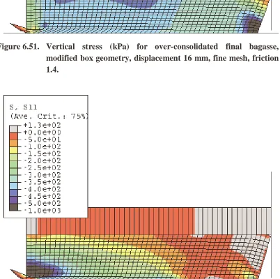
Figure 6.51. Vertical stress (kPa) for over-consolidated final bagasse, modified box

Figure 6.52. Horizontal stress (kPa) for over-consolidated final bagasse, modified box

Figure 6.53. Shear stress (kPa) for over-consolidated final bagasse, modified box geometry,

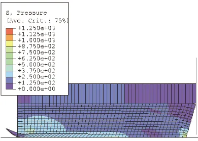
Figure 6.54. Confining pressure (kPa) for over-consolidated final bagasse, modified box

(22)

Figure 6.55. Shear strain for over-consolidated final bagasse, modified box geometry, displacement 16 mm, fine mesh, friction 1.4... 184

Figure 6.56. Void ratio for over-consolidated final bagasse, modified box geometry,

Figure 7.1. Overall geometry of direct shear test at higher pressures. ...188

Figure 7.2. Arrangement of top plate and surface details for higher pressure tests. ...189

Figure 7.3. Compression behaviour of final mill bagasse loaded to a vertical pressure of

15000 kPa...197

Figure 7.4. Shear behaviour of lightly over-consolidated final mill bagasse from a pressure

close to that in a delivery nip... 198

Figure 7.5. Shear behaviour of highly over-consolidated final mill bagasse from a pressure

close to that in a delivery nip... 199

Figure 7.6. Volumetric strain during shearing for prepared cane. ... 201

Figure 7.7. Volumetric strain during shearing for first bagasse. ... 201

Figure 7.8. Volumetric strain during shearing for final bagasse... 202

Figure 7.9. Normalised maximum and final shear stresses for prepared cane...204

Figure 7.10. Normalised maximum and final shear stresses for first bagasse. ...205

Figure 7.11. Normalised maximum and final shear stresses for final bagasse. ...205

Figure 7.12. An estimate of the dilatancy angle for prepared cane. ...207

Figure 7.13. An estimate of the dilatancy angle for first bagasse...208

Figure 7.14. An estimate of the dilatancy angle for final bagasse. ...208

Figure 7.15. Shear stress versus effective vertical pressure for prepared cane...211

Figure 7.16. Shear stress versus effective vertical pressure for first bagasse. ...211

Figure 7.17. Shear stress versus effective vertical pressure for final bagasse. ...212

Figure 7.18. Coefficients of shear versus effective vertical pressure for prepared cane. ....214

Figure 7.19. Coefficients of shear versus effective vertical pressure for first bagasse. ...214

Figure 7.20. Coefficients of shear versus effective vertical pressure for final bagasse...215

Figure 7.21. Coefficients of shear for normally consolidated prepared cane and

over-consolidated prepared cane, first bagasse, and final bagasse...216

Figure 7.22. Maximum shear stress versus effective vertical pressure for prepared cane of

(23)

Figure 7.23. Maximum shear stress at an effective vertical pressure of approximately 1800 kPa for different cane varieties. ... 218

Figure 7.24. Sample height at an effective vertical pressure of approximately 1800 kPa for

different cane varieties. ...219

Figure 8.1. Clay yield surfaces in the p-t plane (after Hibbit et al, 2001). ...225

Figure 8.2. Locations of normal compression, elastic unloading-reloading, and critical state

lines in void ratio – confining pressure plane. ... 226

Figure 8.3. Shape of yield surface for extended Modified Cam Clay with M=1.1 and

β=0.21...228

Figure 8.4. Reproduction of compression behaviour for MCC with β=0.21...229

Figure 8.5. Reproduction of unloading behaviour for MCC with β=0.21...229

Figure 8.6. Reproduction of reloading behaviour for MCC with β=0.21...230

Figure 8.7. Reproduction of shear stress versus shear strain for MCC with β=0.21...231

Figure 8.8. Reproduction of specific volume versus shear strain for MCC with β=0.21..231

Figure 8.9. Definitions of state parameter and critical state constants for material model

CASM (after Yu, 1998)...234

Figure 8.10. Yield surfaces for the MCC and CASM (Yu, 1998) material models...235

Figure 8.11. Potential surface for CASM material model... 236

Figure 8.12. Reproduction of compression behaviour for modification 1 of Yu’s (1998)

model. ... 241

Figure 8.13. Reproduction of unloading behaviour for modification 1 of Yu’s (1998) model.

...242

Figure 8.14. Reproduction of reloading behaviour for modification 1 of Yu’s (1998) model.

...242

Figure 8.15. Reproduction of shear stress versus shear strain for Modification 1 of Yu’s

(1998) model. ...244

Figure 8.16. Reproduction of specific volume versus shear strain for Modification 1 of Yu’s

(1998) model. ...244

Figure 9.1. Pressure feeder of No 1 milling unit on B train at Victoria Mill...249

Figure 9.2. Forces acting on a pair of rolls (reproduced from Murry and Holt, 1967). ....251

Figure 9.3. Loughran and McKenzie pressure vs compression ratio relationship. ...253

Figure 9.4. Fit to Plaza et al (1993) data of pressure vs compression ratio relationship given

(24)

Figure 9.5. Shear stress versus vertical pressure for prepared cane at low vertical pressures (reproduced from Plaza and Kent, 1997)...255

Figure 9.6. Shear stress versus vertical pressure for prepared cane (reproduced from Plaza

and Kent, 1998). ...255

Figure 9.7. Plastic volumetric strain data for Drucker Prager Cap material model

simulations. ...261

Figure 9.8. Initial model geometry for Victoria Mill B1 pressure feeder simulation...262

Figure 9.9. Predicted confining pressure (kPa) for the Victoria Mill B1 pressure feeder. 269

Figure 9.10. Predicted confining pressure (kPa) for the underfeed nip of the Victoria Mill B1

pressure feeder...270

Figure 9.11. Predicted confining pressure (kPa) for the pressure feeder nip of the Victoria

Mill B1 pressure feeder...270

Figure 9.12. Predicted Von Mises stress (kPa) for the underfeed nip of the Victoria Mill B1

Figure 9.13. Predicted Von Mises stress (kPa) for the pressure feeder nip of the Victoria

Mill B1 pressure feeder...271

Figure 9.14. Predicted vertical stress (kPa) for the underfeed nip of the Victoria Mill B1

Figure 9.15. Predicted vertical stress (kPa) for the pressure feeder nip of the Victoria Mill

B1 pressure feeder. ...272

Figure 9.16. Predicted horizontal stress (kPa) for the underfeed nip of the Victoria Mill B1

Figure 9.17. Predicted horizontal stress (kPa) for the pressure feeder nip of the Victoria Mill

B1 pressure feeder. ...273

Figure 9.18. Predicted shear stress (kPa) for the underfeed nip of the Victoria Mill B1

Figure 9.19. Predicted shear stress (kPa) for the pressure feeder nip of the Victoria Mill B1

Figure 9.20. Predicted shear strain for the underfeed nip of the Victoria Mill B1 pressure

feeder. ...275

Figure 9.21. Predicted shear strain for the pressure feeder nip of the Victoria Mill B1

Figure 9.22. Predicted void ratio for the underfeed nip of the Victoria Mill B1 pressure

feeder. ...276

Figure 9.23. Predicted void ratio for the pressure feeder nip of the Victoria Mill B1 pressure

(25)

Figure 9.24. Predicted points where the material is yielding for the Victoria Mill B1 pressure feeder. ...277

Figure 9.25. Predicted void ratio using the Modified Cam Clay material model at a close up

of final bagasse next to the underfeed roll of the Victoria Mill B1 pressure feeder. ...279

Figure 9.26. Predicted void ratio using the Drucker Prager Cap material model at a close up

of final bagasse next to the underfeed roll of the Victoria Mill B1 pressure feeder. ...279

Figure 9.27. Predicted shear stress (kPa) for the top pressure feeder roll and underfeed roll

of the Victoria Mill B1 pressure feeder with back stop not fixed. ...281

Figure 9.28. Predicted shear stress (kPa) for the top pressure feeder roll and underfeed roll

of the Victoria Mill B1 pressure feeder with back stop fixed. ...281

Figure 9.29. Predicted points where the material yielded for the top pressure feeder roll and

underfeed roll of the Victoria Mill B1 pressure feeder with back stop not fixed. ...282

Figure 9.30. Predicted points where the material yielded for the top pressure feeder roll and

underfeed roll of the Victoria Mill B1 pressure feeder with back stop fixed..282

Figure 9.31. Predicted confining pressure (kPa) for aligned top pressure feeder roll and

underfeed roll of the Victoria mill B1 pressure feeder. ...285

Figure 9.32. Predicted Von Mises stress (kPa) for aligned top pressure feeder roll and

underfeed roll of the Victoria Mill B1 pressure feeder...285

Figure 9.33. Predicted vertical stress (kPa) for aligned top pressure feeder roll and underfeed

roll of the Victoria Mill B1 pressure feeder... 286

Figure 9.34. Predicted horizontal stress (kPa) for aligned top pressure feeder roll and

underfeed roll of the Victoria Mill B1 pressure feeder...286

Figure 9.35. Predicted shear stress (kPa) for aligned top pressure feeder roll and underfeed

roll of the Victoria Mill B1 pressure feeder... 287

Figure 9.36. Predicted shear strain for aligned top pressure feeder roll and underfeed roll of

the Victoria Mill B1 pressure feeder. ... 287

Figure 9.37. Predicted void ratio for aligned top pressure feeder roll and underfeed roll of

the Victoria Mill B1 pressure feeder. ... 288

Figure 9.38. Predicted points where the material is yielding for aligned top pressure feeder

(26)

Notation

a , P Position of critical state line _a

β Extension of Modified Cam Clay model

e

D Elastic matrix

ep

D Elastic-plastic matrix E Young’s Modulus

G Shear Modulus

e Void ratio

σ Stress

ε Strain

v Specific volume

λ Slope of normal compression line κ Slope of elastic unloading-reloading line

χ Hardening constant

φcs Equivalent critical state friction angle F Yield surface

Q Plastic potential surface H Plastic hardening modulus

Ko At rest earth pressure coefficient, horizontal effective stress divided by the vertical effective stress

M Slope of critical state line in pressure-shear stress plane

OCR Over Consolidation Ratio, ratio of maximum stress experienced previously to current stress,

c

P ,P Size of yield surface, pre-consolidation pressure, pressure at the intersection _b

of the current elastic loading reloading line with the normal compression line

R Extension of Drucker Prager Cap model d Cohesion for Drucker Prager Cap model p Pressure (or stress)

'

(27)

r spacing ratio for CASM model

n stress state coefficient for CASM model υ Poisson's ratio

C Compression ratio

γ Compaction

f Fibre content

f

ρ Fibre density

j

ρ Juice density

µ Coefficient of friction

θ Angle between line connecting a roll pair and location on the roll surface D Diameter of roll

L Length of roll

G Total torque on one roll

(28)

1

Chapter 1 – The need for a better understanding of bagasse

behaviour

1.1 Introduction – the hypothesis

The project sets out to improve the understanding of the generalised stress-strain relationships (ie. the constitutive equations) that characterise the way in which cane fibres behave during the milling process. Put in more detailed terms, the project seeks to show that bagasse exhibits critical state behaviour, to determine material parameters for prepared cane and bagasse, and to make progress towards a robust material model that can reproduce the compression, shear, and volume behaviour over the range of stresses and strains relevant to the milling process to which sugar cane is subjected.

1.2 Background

The Australian sugar industry is one of Australia’s largest rural industries and one of the world’s largest exporters of raw sugar, contributing directly and indirectly over $4 billion to the Australian economy. The 40 Mt of sugarcane produced in Australia each year generates about $2 billion from the sale of raw sugar, of which about 80% is exported. To remain competitive in the world market, the cost of production of raw sugar has had to continually decrease at a long term average rate of approximately 2% each year (Fry, 1996). Cost reductions have been achieved through growth of the industry to reduce the unit costs of production and through continued research and development to reduce costs and increase the efficiency of the raw sugar manufacturing process.

(29)

Sugar cane is prepared for milling in a hammer mill, which reduces the cane to a mixture of juice, storage cells and lengths of multiple and individual fibres. When freshly prepared, this is quite similar to moist straw, but when handled it is not readily apparent that there is a high level of moisture (mass of water divided by total mass equal to 70%) in the material (shown in Figure 1.2). This prepared cane is then compressed between pairs of rollers in a six roll milling unit to extract the maximum possible quantity of sugar juice. The solid material leaving this milling unit is called bagasse. The bagasse is then sprayed or soaked with dilute juice and then passed through up to five further mills, in a counter current extraction process, with a further spraying or soaking process occurring before each subsequent mill (the initial hot water is usually added just before the final milling unit). The final bagasse (shown in Figure 1.3), still containing about 2% sugar and 50% water (mass divided by total mass), is then burnt to provide self-sufficient power to the factory.

Improved juice extraction performance has benefits in terms of increased sugar production and results in lower moisture fuel and hence higher boiler capacity for steam generation. Milling units and boilers have the highest capital costs of any individual items of sugar factory plant.

(30)

Figure 1.2. Prepared cane.

(31)

Increases in mill and boiler capacity through improved operational settings will have significant financial benefit to the industry. Incremental milling capacity has a capital cost of about $100,000 for every tonne of cane per hour increase in capacity, so there is a substantial incentive for the industry to improve the capacity of existing mills without the need for new capital expenditure. An avenue for improved performance is through computer modelling. Based on the experience gained from the modelling of other factory processes, for example, clarifier modelling (Steindl, 1995, Steindl et al., 1998) and boiler modelling (Dixon and Plaza, 1995, Plaza et al., 1999), it is expected that improved modelling of the milling process will result in increased throughput through existing milling units and improved juice extraction performance.

The milling process consists of three distinct but coupled phenomena: 1. The fibrous skeleton of the prepared cane or bagasse is subjected to pressures from typically 2 kPa to 20 MPa. This results in large compressive and shear strains that reorient, distort and break the fibres. 2. The juice flows within the porous matrix of this skeleton at rates governed by the void ratio and therefore its degree of compression and pressure differential. 3. Juice flows through the boundaries of the bagasse, where compressive and frictional stresses are applied. The interaction of all these processes influences the roll loads, the roll torques, and the percentage juice extraction.

1.3 Previous work on the milling process

(32)

In 1989 the Sugar Research Institute in Mackay and the Sugar Research and Development Corporation began funding the development of a milling model at the University College of Swansea in Wales. The milling model was to incorporate the fundamental equations that describe the mechanisms occurring in the milling process. The development of the model of a two roll mill by Zhao (1993) and Owen et al. (1995) at the University College of Swansea involved the use of porous media mechanics and finite element methods to describe the behaviour of prepared cane. The model is based on the governing equations for saturated - unsaturated porous media and has been simplified somewhat by assuming that accelerations can be neglected. Darcy's law is used to describe the flow of the juice through the fibrous skeleton. The bagasse has a degree of water saturation of at least 85% at most of the locations in a milling unit, except at the feed chute and underfeed rolls, and after the delivery nip. A significant amount of air is also present in the bagasse at feed chute conditions. Terzaghi's principle of effective stress is assumed to apply. The material is essentially described with a two-phase model, consisting of the fibrous skeleton and the juice.

(33)

Crucial to this model is a suitable material (constitutive) description for the stress-strain behaviour of the fibrous skeleton. The model developed by Zhao (1993) used a linear elastic material model that was unsuitable for bagasse, which experiences large unrecoverable strains when loaded. The lack of a suitable material model has hindered the development and application of the finite element model to real milling situations. A more suitable family of material models applicable to bagasse, called critical state models, was identified by Leitch (1996) and adopted by Adam (1997). Further development of Zhao's model was undertaken by Zhao at Swansea and Adam (1997) at James Cook University. The development of the model has been monitored and assessed periodically, for example, by Edwards et al. (1995) and Kent et al. (1998).

1.4 Explanation of the critical state concept

Critical state models were developed for saturated soils, which are similar (to a degree) to prepared cane, in that they exhibit elastic and plastic behaviour, large strains and compressive behaviour at yield. Prepared cane is also saturated with water at many locations in a milling unit. The critical state models had their origin at the Cambridge Soil Mechanics Group in the United Kingdom, see Roscoe et al. (1958), Schofield and Wroth (1968), Atkinson and Bransby (1978), following and building on the measurements carried out by Rendulic (1936) and Henkel (1960). Further development and description of critical state models in soil mechanics is given, for example, in Britto and Gunn (1987) and Muir Wood (1990). Critical state models unify the compression, shear and volume behaviour of soils. Critical state models are formulated in three dimensional p:q:v space where p is the average of the normal stresses acting on the body, q (the deviatoric axis) is related to the shear stresses, and v is the specific volume (or some other appropriate volumetric measure such as e, the void ratio). Constitutive models of particular interest have been the Modified Cam Clay (MCC) model, the Crushable Foam model and the Drucker-Prager Cap (DPC) model.

(34)

not be repeated here. A short description of the relevant features is given below. Extensions of the MCC and DPC models are described in Chapter 8.

Figure 1.4 shows the plastic and elastic compression behaviour in the p:e plane. Initial loading takes place along the normal compression line (NCL), also known as the normal consolidation line, and is shown in Figure 1.4 as the line with a plastic slope. The unloading and reloading behaviour takes place along the elastic line that is shown in Figure 1.4 as the line with an elastic slope. When reloading along the elastic line reaches the NCL it continues along the NCL line. At a relatively low level of unload (the ‘wet’ side of critical state) the material will decrease in volume during shearing. At a relatively high level of unload (the ‘dry’ side of critical state) the material will increase in volume during shearing. Between these two extremes is the location of the critical state where no change in volume or stress occurs with ongoing shear deformation (not shown in Figure 1.4).

(35)

When viewed in the p:q plane, the Modified Cam Clay critical state model has an elliptical yield surface (see Figure 1.5, where q is given as t, following Hibbit et al., 2001), and an associated plastic flow rule, which defines the plastic strain vector as being orthogonal to the point on the yield surface intersected by the material's stress path. The plastic strain vector has two components: the plastic volumetric strain parallel to the p axis, and the plastic shear or shape strain parallel to the q axis. Critical state occurs at the apex of the ellipse, where there is (ongoing) shape change at constant volume and stress. The material’s hydrostatic pressure-volume relationship (the normal compression line) governs the growth and contraction of the yield surface. The shape of the elliptical yield surface is dependent on M, the slope of the critical state line in the p:q plane. The M parameter is normally obtained by taking the material to critical state in a triaxial test, or is estimated in direct shear box tests. An extension of the Modified Cam Clay model is given in Hibbit et al. (2001) whereby the shape of the yield surface (in particular, the right hand side of the ellipse) can be further modified by the use of a β parameter.

(36)

The Crushable Foam model was developed for the analysis of materials such as foams and honeycombed structures. It is a variation on the Modified Cam Clay model. It uses a non-associated elliptical flow potential centred about the deviatoric stress axis. This flow potential is based on the observation of negligible radial plastic strains in simple compression tests. ‘Associated’ means that (post-yield) flow is perpendicular to the yield surface. ‘Non-associated’ means the flow is not perpendicular to the yield surface.

The Drucker-Prager Cap model has an elliptical yield surface on the ‘wet’ side of critical state, and a Mohr-Coulomb type shear failure surface on the ‘dry’ side (shown in Figure 1.6). The elliptical yield surface has an associated flow rule governing the plastic strain vector, whilst the shear failure surface has non-associated flow, that is the plastic strain vector is non-associated with another potential surface which intersects the yield surface at the point where the material has commenced plastic flow.

(37)

Leitch et al. (1997) carried out a search of available constitutive models including isotropic elasticity, isotropic elasto-plastic models and anisotropic models. They concluded that anisotropic models were too complex at the time to be coded into a computer model and recommended the model for coding to be a modified isotropic associated flow Crushable Foam model. Adam (1997) discontinued the use of the Crushable Foam plasticity model due to severe numerical convergence difficulties and used the Drucker-Prager Cap and Modified Cam-clay models such that they basically represented the same model by using an inverse calibration procedure based on uniaxial compression tests. Loughran and Adam (1998) presented an inverse calibration procedure using the Drucker-Prager Cap plasticity model in combination with uniaxial compression tests to determine material parameters such as M, the slope of the critical state line.

1.5 Experimental investigation of critical state models

The yield surfaces and plastic flow rules of Modified Cam Clay and Capped Drucker-Prager models were developed after extensive testing of soil samples in p:q:v space (Schofield and Wroth, 1968; Muir Wood, 1990; Hibbitt et al, 2001). Numerous stress probes were carried out to define the yield surfaces, and ascertain the direction of the plastic strain vectors.

(38)

Leitch concluded that, for the purpose of developing a material model, ‘the test results were considered to be unreliable’. Therefore, although critical state material parameters have been obtained by several investigators from analysing the deviatoric part of the triaxial tests as reported below, these parameters must be treated with a great deal of caution.

1.6 Derivation of critical state parameters

Loughran and Adam (1998) and Owen et al. (1998) summarised their derivations of the parameters of prepared cane. In order to improve their predictions of simple uniaxial compression, the parameter M (slope of the critical state line) was set at 3.8 to 4.0. This range of values was stated to be derived from inverse calibration of uniaxial test data and from the Leitch (1996) triaxial results. It is noted that values of M as high as 3.8 and 4.0 imply physically impossible friction angles. A maximum value for M is 3.0, for which the corresponding friction angle for triaxial compression is 90 degrees. Following Carter (2003), the physical absurdity of values of M of 3.8 and 4.0 is noted. However, since these values have been extensively used in many modelling papers, it has been necessary in this investigation to address the use of such values and the results of their use.

Kirby (1997) calculated estimates of M from the Leitch data to be from 0.07 to 2.0. Schembri et al. (1998) concluded that, on the basis of the Leitch data, ‘M is unlikely to be greater than 2 and may be much less’. Considering the above, and Leitch’s own conclusions on the quality of the measured data, it is unlikely that a value of M can be obtained with confidence from the Leitch (1996) data. Kirby (1997) calculated M values of about 1.0 as derived from direct shear box tests of Plaza and Kent (1997). The value of M used in the Drucker Prager Cap (or the MCC) material model has important implications for the kind of material behaviour that a milling model can reproduce. There is a major discrepancy between the values of M quoted by Loughran and Adam (1998) and Owen et al. (1998) and those quoted by Kirby (1997) and Schembri et al. (1998).

(39)

model as calibrated by Loughran and Adam (1998). These modelling tests concluded that adjustments to the M value can be used in some situations (such as uniaxial compression loading) to improve the predictions to the detriment of other predictions (such as loading in shear). This suggests that the model and procedure adopted by Loughran and Adam is suited to only a narrow range of stress states, and should be viewed with caution when considering its application to a milling simulation, which is believed to involve complex stress conditions. Although large portions of the milling process are believed to subject the fibrous skeleton to uniaxial compression, there is also evidence that there are locations in a mill in which the bagasse experiences significant shear strains (Plaza and Kent, 1997, Schembri et al., 1998). Chapter 5 in this investigation describes a limitation in the MCC and DPC models that explains the reason for the above modelling problems.

1.7 Inverse methods for obtaining material parameters

The inverse method topic for obtaining material parameters is touched upon because it has been referred to, used by, and modified, by several authors in the milling research field in the last 10 years. Zhao (1993) adopted this approach when confronted with the fact that a constitutive relationship relating stresses and strains (a material model) was not available for bagasse. He refers to previous work on inverse methods including Mehta (1984), Kubo (1988), Maniatty and Zabaras (1989), Zabaras and Ruan (1989) and Schnur and Zabaras (1990).

Zhao developed an inverse problem solution to an experimental compression stress versus strain curve (a normal compression line in soil mechanics terms) supplied to him by the Sugar Research Institute. It is noted that there seems to have been an error made in what this compression curve represented because Zhao stated that ‘this curve is very different from the stress-strain curves for other porous media (e.g. soil, concrete)’. However, the supplied curve is actually very similar to the normal compression line observed in soil tests.

(40)

1.7) (it is noted that the Swansea research reports are compiled in the appendices of Garson, 1992b). The curve is reproduced here in Figure 1.8 with the stress plotted on a natural log scale (basically the normal compression curve usually plotted in soil mechanics, except strain is plotted instead of specific volume or void ratio, and therefore the slope of the line is reversed). A linear relation is evident, as is the case for soils (see, for example, Figure 4.20 in Craig, 1987). The result provides strong evidence that the behaviour of prepared cane in uniaxial compression is very similar to that of soils.

(41)

Zhao commented that no constitutive relation exists for bagasse but then stated that ‘the form of the constitutive relations for other porous materials such as soil and concrete is far removed from that needed for prepared cane’. The same statement is made by Owen at al. (1994a) and Owen et al. (1995). However, no details of results or references were given to justify the statement. These statements are believed to be the result of the error made in what the compression curve represented, and the resultant erroneous conclusion that the behaviour of prepared cane is very different from that of soil. Experimental evidence is provided in Chapters 3, 4 and 7 of this thesis that shows that the form of the constitutive relations for prepared cane are quite similar to those for soil.

Over the following eight years the use of uniaxial compression tests and inverse calibration procedures was emphasized (Owen et al., 1994a, Owen et al., 1994b, Owen et al., 1995, Loughran and Adam, 1995, Adam, 1997, Adam et al., 1997a, Adam et al., 1997b, De Souza Neto et al., 1997, Adam and Loughran, 1998,

y = 0.151Ln(x) + 0.201

R2 = 0.9989

0.0 0.1 0.2 0.3 0.4 0.5 0.6 0.7 0.8

1 10 100

Stress (MPa)

Stra

in

(42)

Loughran and Adam, 1998, Owen et al., 1998, Downing, 1999, Downing et al., 1999a, Downing et al., 1999b, Loughran and Kannapiran, 2002).

Indeed, De Souza Neto et al. (1997) stated that ‘Before the developed computational tool can be applied to industrial simulation, a necessary prerequisite is identification of the material parameters of the solid phase by numerical experiments, since it is impossible to undertake material tests on samples in the dry state. Therefore, an inverse procedure in which the material properties of the solid phase are deduced by computationally replicating the actual experimental material tests must be undertaken’. The statement is repeated in Owen et al. (1998). However, it is believed to be incorrect. Tests to obtain material parameters (for example, triaxial tests, direct shear tests, ring shear tests, vane tests) have been carried out for soils over at least the last 100 years on materials that are wet, whether the materials are drained or not, saturated or not and both in the laboratory and the field, without the need for an inverse calculation procedure (see for example, Craig, 1987, Muir Wood, 1990).

Most of the literature on the solution of inverse problems (Mehta, 1984, Kubo, 1988, Maniatty and Zabaras, 1989, Zabaras and Ruan, 1989, and Schnur and Zabaras, 1990) has been devoted to inverse heat transfer problems, with some other application to static elastic problems. Inverse methods are still in their infancy in terms of development and in comparison to, for example, the material parameter development work carried out in the soil mechanics field. In combination with the material parameter development work, inverse analysis methods have been applied in the soil mechanics field for example by Kirby et al. (1998) and Kirby (1998b), and have recently been applied to prepared cane and bagasse (Kent, 2001; Plaza et al., 2001).

(43)

1.8 The current state of material models for prepared cane

The situation at the middle of 1998 was that the Drucker-Prager Cap model had been successfully used to predict some of the empirical trends relating to roll loads, roll torques and juice extraction in a milling unit, but not some others and not together in a simulation using the same parameters. Its inability to model some known aspects of the fibrous skeleton behaviour left concern that the model did not capture some important mechanisms and hence could not lead to an improved understanding of the milling process. To resolve this doubt, an improved material model for the fibrous skeleton and improved methods of determining parameters for the material model are required. Prepared cane has been fitted into the critical state models Modified Cam Clay and Drucker-Prager Cap by manipulation of the parameters, but a reliable and consistent material model has not been achieved. Indeed, all experimental test methods up to this time have failed to measure the basic behaviour for prepared cane or bagasse which is required to develop a reliable critical state model, or even to identify bagasse as a critical state material (as shown for soil, for example, in Craig 1987, Muir Wood 1990). Although the parameter M has been used as an example, there are many other parameters that require identification (such as the position of the critical state line relative to the normal consolidation line) in order to build a reliable critical state model for bagasse.

1.9 Review of available test methods to measure critical state behaviour

(44)

from deviatoric tests are not available either for normally consolidated samples or over-consolidated samples.

The direct shear test method is less time consuming and less expensive than the triaxial test. It is widely used to test frictional materials, i.e. sands. Its drawbacks are that the full stress state is not known and it does not allow the measurement of pore water pressure. However, it is very successfully used in soil mechanics engineering and design in combi