1
Integrated Structural Analysis Tool using the Linear Matching
Method part 2 – Application and Verification
Haofeng Chena,, James Urea, David Tippingb
a
Dept of Mechanical and Aerospace Engineering, University of Strathclyde, 75 Montrose
Street, Glasgow G1 1XJ, Scotland, United Kingdom
b
Central Engineering Support, EDF Energy Nuclear Generation Ltd., Barnwood, Gloucester
GL4 3RS, United Kingdom
Abstract
In an accompanying paper, a new integrated structural analysis tool using the Linear Matching Method framework for the assessment of design limits in plasticity including load carrying capacity, shakedown limit, ratchet limit and steady state cyclic response of structures was developed using Abaqus CAE plug-ins with graphical user interfaces. In the present paper, a demonstration of the use of this new Linear Matching Method analysis tool is provided. A header branch pipe in a typical advanced gas-cooled reactor power plant is analysed as a worked example of the current demonstration and verification of the Linear Matching Method tool within the context of an R5 assessment. The detailed shakedown analysis, steady state cycle and ratchet analysis are carried out for the chosen header branch pipe. The comparisons of the Linear Matching Method solutions with results based on the R5 procedure and step-by-step elastic-plastic finite element analysis verify the accuracy, convenience and efficiency of this new integrated Linear Matching Method structural analysis tool.
Keywords: Linear Matching Method , Load Carrying Capacity, Shakedown limit, Ratchet limit,
Steady State Cycle, Pipe Header
2
1.
Introduction
Many engineering structures and components subjected cyclic thermal and mechanical loads experience alternating plasticity leading to low cycle fatigue (LCF) or ratchetting which results in an incremental plastic collapse. The evaluation of the LCF, shakedown and ratchet limits have been researched and modelled extensively by plasticity theorists, materials scientists, mathematicians and engineers. Cyclic plasticity is a complex problem and in recent years significant advances have been made in characterising different responses. Incremental Finite Element Analysis provides a powerful tool to simulate the elastic-plastic behaviour of structures subjected to a specified load history. This allows investigation of any type of load cycle but also requires significant computer effort for complex 3D structures. In addition, this approach does not predict a shakedown or ratchet limit, it simply shows whether elastic shakedown, plastic shakedown or ratchetting occurs. To calculate the specific shakedown or ratchet limit, a significant number of simulations at different load levels are required to establish the boundary between shakedown and non-shakedown behaviours. The designer ideally requires a shakedown/ratchet analysis method that (i) can be applied efficiently to complex 3D geometry under complex thermo-mechanical loading, (ii) only requires readily available computing facilities and (iii) unambiguously specifies shakedown and ratchet limits.
Hence adopting both the upper and lower bounding theorems [1, 2], direct methods [3-8] have been developed to directly address the limit load, shakedown and ratchet limits required in a design situation. However, shakedown and ratchet analyses are often difficult to incorporate in a design process. Typically these advanced direct methods require specialist programs that are not available or supported commercially and the computing required to analyse practical structures is extensive and often impractical. In the absence of a robust and practical plastic analysis method, design for shakedown in practice is still based on simple solid mechanics models incorporating design factors sufficient to ensure an adequate “margin of safety” against ratchetting is present [9]. This often leads to excessive conservatism in a design, with obvious technical and economic implications.
3 capacity to be implemented easily within a commercial finite element code, Abaqus [19]. The LMM provides a general-purpose technique for the evaluation of shakedown and limit loads, ratchet limit, plastic strain range for the low cycle fatigue (LCF) assessment associated with a steady state cycle.
To enable widespread adoption of the LMMs in industry, an integrated software tool is further developed to not only removes the requirement for manual subroutine alterations, but also provide additional functionality for subsequent life assessment calculations. In an accompanying paper [20], this new integrated structural analysis tool using the LMM framework for the assessment of load carrying capacity, shakedown limit, ratchet limit and steady state cyclic response of structures was presented, and this new software tool will serve two functions.
4 described in section 4. The setup and submission of the LMM analysis of the header is presented in section 5, followed by a comparison of results with the R5 and incremental elastic-plastic finite element analysis (FEA) results.
2.
Problem background and description
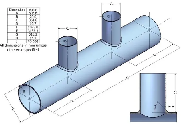
A schematic of such a header is shown in Figure 1, where the main pipe has two parallel branch pipes. There are a number of these secondary headers in the system. They have all been designed with the same wall thicknesses, but two variations exist with regards to the distance between two branch pipes.
Non-destructive testing (NDT) was performed on a number of headers to determine current wall thicknesses. This inspection showed a significant variation in these wall thicknesses, where the minimum main and branch pipe thicknesses were found to be 20mm and 10.7mm respectively. It should be noted that these minimum thicknesses were not observed in the same header.
In order to prove shakedown in all of the headers whilst keeping the number of analyses to a minimum a worst case model was created. The minimum wall thicknesses observed from the NDT of all the headers were used in this model despite their occurrence in different headers. This gives an inherent conservatism in the model.
This worst case model also considered the possibility of an interaction between two branch pipes. There are two header geometries, the difference between them being the dimension F (3153.3mm and 4169.3mm) in Figure 1. It was shown in [21] that the smaller of these two designs could show an interaction of stresses between two branches whereas the larger design would not. Therefore as a conservative approach the smaller branch geometry was used.
The design conditions of the header are an internal pressure of 4.55MPa, which is limited by a safety relief valve upstream of the header, and a temperature of 382.2oC. The analysis assumes that the pipework operates between two relatively steady state conditions of cold shutdown and hot pressurised, which was confirmed by plant temperature and pressure data. Therefore no cold-pressurised or thermal shock conditions are considered.
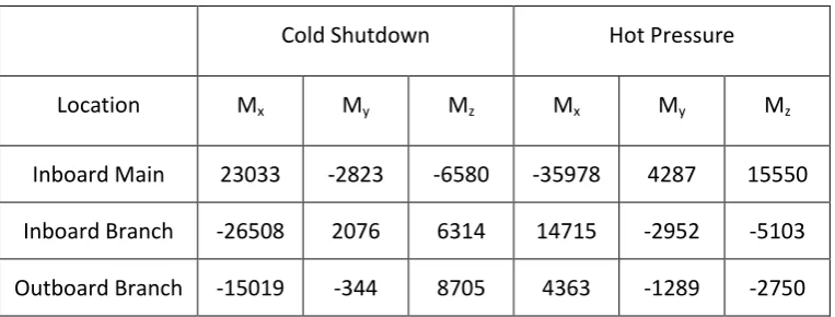
5 software PSA5 [22] for the entire cold reheat piping system. There was a variation in bending moments seen across all the headers in the system, and so the worst case bending moments were chosen as a conservative option for this model.
3.
Finite Element Model
3.1.
Geometry
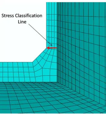
The dimensions of the header geometry used are shown in Figure 1, and the model and mesh are created to match that of [21] as closely as possible. The weld is modelled as a 45 degree chamfer with a leg length of 14.1mm. This gives a weld cap dimension of 20mm, which was the minimum observed in the inspection data. Although symmetry exists in this geometry, the applied bending moments are not symmetrical. Therefore symmetry could not be used.
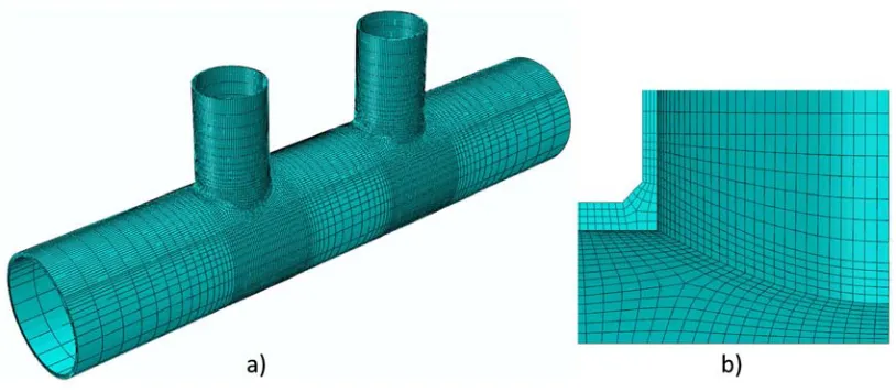
The FE model is meshed with the Abaqus quadratic brick element C3D20R, as shown in Figure 2a. The mesh is biased to be denser in the region of the intersection and weld, resulting in a total of 52240 elements in the model. The weld region is meshed as shown in Figure 2b, which results in no element warnings for internal angles or aspect ratio.
3.2.
Material Properties
Table 1 shows the young’s modulus and yield stress at 20oC and 382.2oC, respectively. For a shakedown assessment R5 also includes a factor, Ks, on the yield stress. This represents the ability of material to harden or soften during repeated cycles of loading. The header pipework is produced from BS-3602-HFS-27S carbon steel. The Ks factor for carbon steels given in R5 is 0.73 at 20oC and 0.9 for temperatures above 150oC. This gives the shakedown yield stresses in Table 1, where the value of Ks (<1) corresponds to cyclic softening.
3.3.
Loads and Boundary Conditions
The internal pressure of 4.55MPa is applied to all internal surfaces of the model. The closed end condition is replicated by applying the equivalent axial tension to the ends of the main and branch pipes. Two temperature extremes of 20oC and 382.2oC are assumed to be entirely uniform with no temperature differences within the model. Therefore these are modelled using uniform predefined fields.
6 here is the same as [21]. In all cases these constraints allow for radial expansion of pipes due to internal pressure.
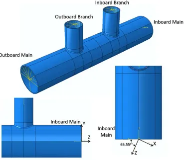
The worst case bending moments from the PSA5 analysis are given in Table 2. The PSA5 analysis has its own global co-ordinate system which differs from that of Abaqus. Therefore a Cartesian coordinate system was created in at the Inboard Main reference point so that the moments from PSA5 could be directly applied to the model. This coordinate system is shown in Figure 3. The model is constrained by fully fixing the Outboard Main Reference Point in all degrees of freedom.
4.
Previous Shakedown Analysis
To perform the R5 Volume 2/3 [9] shakedown calculations stresses need to be linearised across the section in question. In [21] the stress classification line shown in Figure 4 proved to be most severe, and so those results are presented here. This line is at the outboard side of the inboard branch pipe.
4.1.
R5 Simple Checks
Checks in R5 Volume 2/3 were used to determine the shakedown status of the component, beginning with the simple checks in R5 section 6.6. This check assumed that the residual stress field is null. The shakedown condition is met if the linearised elastic stresses
ˆ
e are less than the modified yield stress:
e
x t
K
s yˆ
,
(1)where σy is the minimum 0.2% proof stress of material and Ks is the factor applied to σy to
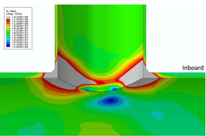
obtain material ratchet limit. An elastic analysis was performed for the cold shutdown and hot pressurised states. Figure 5 shows a contour plot of the von-Mises equivalent stress at the hot-pressurised condition, where the contour limit has been set to the shakedown yield stress of 125.7MPa. It can be seen that a significant region around intersections has exceeded this limit, shown in grey. The linearised stresses across the classification line in Figure 4 exceed the yield stress: the von-Mises equivalent membrane + bending stress at the inner and outer surfaces are 278MPa and 246MPa respectively. This is in excess of the modified yield and so shakedown cannot be demonstrated using a simplified check.
4.2.
R5 Shakedown Check Involving a Residual Stress Field
7 The internal pressure and associated axial tensions were applied along with the hot moments to generate the elastic-plastic response at this state. Following this plastic deformation, all the loads were removed which left the resultant residual stress field shown in Figure 6.
When this route is adopted in R5 the stress across the section (including the residual stress field) must satisfy
,
s
x t
K
s y (2)where s is the sum of the applied elastic and residual stresses. If s is a linearised stress distribution, as was used in [21], then equation (2) must be satisfied over the entire classification line. The superposition of the elastic and residual stresses at the hot pressure condition resulted in membrane + bending stresses of 183MPa and 188MPa at the inner and outer surfaces respectively. This is greatly in excess of Ksσy (125.7MPa) at 382.2oC and so fails the shakedown criteria of R5.
4.3.
Elastic-Plastic FEA
Exhaustion of the simplified criteria in R5 meant that cyclic elastic-plastic FEA was required to demonstrate shakedown. An elastic perfectly-plastic material was used with the unmodified yield stresses at 20oC and 382.2oC. The model was cycled between two states of cold shutdown and hot pressure. Figure 7 shows plastic strain contours at the steady state cycle and highlights the location of peak plastic strain (in the branch side weld toe in the inboard branch). The plastic strain in this most critical location is also plotted in Figure 7. It can be seen that the plastic strain stabilises after the first cycle and so the header is within strict shakedown.
5.
Analysis using the LMM software tool
This header branch is re-analysed using the newly developed LMM tool. Steps used in this section to construct the LMM analysis are detailed so as to act as a worked example of a LMM analysis. Results are then compared to the analysis conducted by an industrial partner.
5.1.
Strict Shakedown Analysis
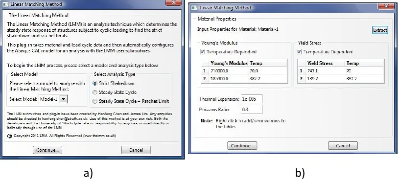
8 Only one material is defined in this model, therefore a single material properties dialog is shown. Figure 8b shows the materials dialog with temperature dependent properties. Only two temperature dependent properties are used so the third row of tables is deleted. The Young’s modulus and Poisson's ratio were already defined for the elastic analysis, and so the “Extract” function was used to populate the dialog box. The elevated temperature in the model is uniform and so no thermal stresses will be generated. Therefore an arbitrary thermal expansion coefficient is entered.
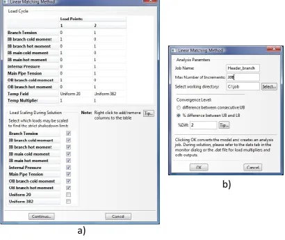
Figure 9a shows the Load Cycle dialog box. The load cycle for this component is assumed to vary between the two conditions of cold shutdown and hot pressure. Therefore two points in the load cycle table are required. The cold moments are applied with a multiplier of 1.0 in the first load instance along with the 20oC temperature field. The hot moments, internal pressure and axial tensions associated with this are not applied and so have a multiplier of zero. In the second load instance, the cold moments have a multiplier of zero. The hot moments, internal pressure and its associated axial tensions are given a multiplier of 1.0. The second load instance is given the 382.2oC temperature field. All loads are allowed to be scaled during the solution. Therefore the resulting shakedown load multiplier will be the level by which all these loads can be scaled to be exactly at the shakedown limit. The two temperature fields are not included in this scaling, which means that yield stresses at both load points will remain unaffected.
The final dialog, shown in Figure 9b, is used to name the analysis, set the working directory, and specify the number of increments and convergence. This is a relatively large model and so a maximum of 300 increments was set. If convergence has not occurred in this time then the analysis is terminated to prevent files becoming too large. A 2% difference between lower and upper bounds was chosen as the convergence tolerance. This value is assumed sufficient to ensure converged lower and upper bounds without allowing the solution time to become excessive.
With the data entered into the dialog, the LMM scripts configure the model as described in section 4 of the accompanying paper [20]. The analysis job is created in CAE, and the model is ready for a LMM analysis. At this point the job definition created by the LMM was modified to solve on multiple CPUs, and then it was submitted for analysis.
9 loads could be increased by approximately 10% whilst still achieving strict shakedown. This result confirms that the header is in strict shakedown as observed in the cyclic elastic plastic FEA. Figure 11 compares contour plots of plastic strain predicted by the LMM and elastic plastic FEA with the same measure of plastic strain. The LMM results are given at the strict shakedown limit, and the Abaqus cyclic elastic plastic FEA results are for the specified loading. Nevertheless, a good agreement is observed.
The elastic plastic analysis of [21] described in section 4.3 used the unmodified yield stress to prove shakedown, and this has been validated with the LMM analysis using the same values of yield stress. However the R5 assessments use a modified value of yield to account for cyclic softening. Header components see a very low number of cycles – plant data shows around 6 cycles per year. Therefore it is questionable whether the steel would see enough cycles to soften by any significant level. Nevertheless it is prudent to check the shakedown status using
K
s y.The LMM analysis was repeated using the shakedown yield stresses from Table 1. The resulting lower and upper bound shakedown multipliers are 0.867 and 0.886 respectively. Therefore the header is not in strict shakedown and further analysis is required to ensure that it is not ratchetting.
5.2.
Steady State Cycle and Global Shakedown Limit
Since strict shakedown could not be achieved when the
K
s yvalues of yield stress were used, the model must either be in global shakedown or ratchetting. To find out which, the model was analysed using the LMM global shakedown procedure. The LMM plug-in was started once again within Abaqus CAE. Figure 12 shows the Main and Material dialog boxes, which are nearly identical to that of the strict shakedown analysis. In this case, the Ramberg-Osgood model is not used due to lack of material data.10 associated axial tensions were selected to be added in stage 2, shown in Figure 13a. This means that the ratchet limit multiplier will correspond to the level of additional pressure loading that will not cause ratchetting. If it was deemed that the safety margin against an increase in cold or hot moments was needed, then these could be selected instead.
The global shakedown analysis required two convergence values. A steady cycle convergence value of 1e-4 was used to obtain a stabilised cycle. A 5% difference in lower and upper bound was chosen for stage 2 in order to reduce the number of increments required. Figure 13b shows the Job dialog box. The model was then solved.
The lower and upper load multipliers given by this analysis were 0.024 and 0.087 respectively, which correspond to an allowable increase in pressure of 2.4% and 8.7% respectively. This means that an increase in pressure of 0.4MPa (using the upper bound multiplier) can be sustained before ratchetting. The difference in load multipliers is greater than 5% specified in the plug-in and is a result of the analysis being terminated due to the size of results files, which were becoming large. The purpose of the stage 2 analysis was to demonstrate if the header is in global shakedown, therefore any positive load multiplier indicates this. Examining load multipliers during the solution shows that the upper bound has converged very well, with little change seen between consecutive increments. The lower bound showed a slow convergence with the inboard branch weld toe being the source of the problem. Despite this, the lower bound shows that at least 0.11MPa of internal pressure can be added before ratchetting will begin and continued solution would approach the converged upper bound value. Based on this the header was judged to be within global shakedown and the analysis was terminated.
11 The second elastic plastic analysis was conducted to validate the location of the global shakedown limit predicted by stage 2 of the LMM calculation. This analysis considered an increase in the internal pressure and tensions of 9%, taking the load cycle just beyond the global shakedown limit predicted by the LMM upper bound. Figure 15 shows the plastic strain history, which shows an accumulation of plastic strain until a plastic hinge forms during the 12th cycle and the analysis halts.
These analyses show that the header operates in global shakedown, but is very close to the global shakedown limit. A relatively small increase in the pressure would result in ratchetting behaviour. Despite this, further evidence to substantiate the global shakedown status of the component comes from available material properties, showing significant work hardening behaviour in this material, which is not taken into account in any of the analyses conducted here. If a Ramberg-Osgood model were available then this could be used in stage 1 of the global shakedown calculation. This hardening would bring the header further away from the global shakedown limit (possibly even to within strict shakedown) which supports the global shakedown status of the header.
6.
Conclusions
This paper has revisited the analysis of a header branch pipe performed by an industrial partner. The original analysis of this component used the R5 procedure, but these checks could not demonstrate that the header was in shakedown. Elastic plastic analysis was performed and showed that the header was in strict shakedown.
The LMM has been used in this paper to re-analyse the header. This provides a worked example of the newly created LMM plug-in software tool. The steps involved in running the LMM strict shakedown analysis and the outputs it produces are described. The LMM results concur with that of the incremental elastic plastic analysis, which show that the header is in strict shakedown when the unmodified yield stress is assumed. However strict shakedown is not achieved if the R5 Ks factor is applied.
12 paper has demonstrated that the developed LMM software tool is capable of solving practical engineering problems with complicated thermal and mechanical load history.
Acknowledgments
The authors gratefully acknowledge the support of the Nuclear EngD Centre of the United Kingdom, EDF Energy and the University of Strathclyde during the course of this work. The authors would also like to thank Prof Alan Ponter from University of Leicester for his advices and discussions on the theoretical and software developments of the LMM.
References
[1] Melan E. Theorie statisch unbestimmter systeme aus ideal-plastichem baustoff. Sitzungsber. d. Akad. d. Wiss 1936; 145(2A): 195–218.
[2] Koiter WT. General theorems for elastic plastic solids. in Progress in solid mechanics, J. Sneddon and R. Hill, Eds. Amsterdam 1960; 167–221.
[3] Vu DK, Yan AM, Nguyen-Dang H. A primal–dual algorithm for shakedown analysis of structures. Computer Methods in Applied Mechanics and Engineering 2004; 193: 4663–4674.
[4] Muscat M, Mackenzie D, Hamilton R. Evaluating shakedown under proportional loading by non-linear static analysis. Computers & Structures 2003; 81: 1727–1737. [5] Adibi-Asl R, Reinhardt W. Non-cyclic shakedown/ratcheting boundary determination –
Part 1: Analytical approach. International Journal of Pressure Vessels and Piping 2011; 88: 311–320.
[6] Staat M, Heitzer M. LISA a European Project for FEM-based Limit and Shakedown Analysis. Nuclear Engineering and Design 2001; 206: 151–166.
[7] Spiliopoulos KV, Panagiotou KD. A direct method to predict cyclic steady states of elastoplastic structures. Computational Methods in Applied Mechanics and Engineering 2012; 223-224: 186-198.
13 [9] R5: An assessment procedure for the high temperature response of structures,
Revision 3. British Energy Generation Limited, Gloucester, UK, 2003.
[10] Ponter ARS, Carter KF. Shakedown state simulation techniques based on linear elastic solutions. Computer Methods in Applied Mechanics and Engineering 1997; 140: 259– 279.
[11] Ponter ARS, Engelhardt M. Shakedown limits for a general yield condition: implementation and application for a Von Mises yield condition. European Journal of Mechanics - A/Solids 2000; 19(3): 423–445.
[12] Chen HF, Ponter ARS. Shakedown and limit analyses for 3-D structures using the linear matching method. International Journal of Pressure Vessels and Piping 2001; 78: 443– 451.
[13] Chen HF. Lower and Upper Bound Shakedown Analysis of Structures with Temperature Dependent Material Properties. ASME Journal of Pressure Vessel Technology 2010; 132(1): 011202.
[14] Chen HF, Ponter ARS. A Direct Method on the Evaluation of Ratchet Limit. ASME Journal of Pressure Vessel Technology 2010; 132(4): 041202.
[15] Chen HF, Ure J, Tipping D. Calculation of a Lower Bound Ratchet Limit Part 1 - Theory, Numerical Implementation and Verification. European Journal of Mechanics - A/Solids 2013; 37: 361-368.
[16] Chen HF, Ponter ARS. Linear matching method on the evaluation of plastic and creep behaviours for bodies subjected to cyclic thermal and mechanical loading. International Journal for Numerical Methods in Engineering 2006; 68(1): 13–32. [17] Chen HF, Ponter ARS, Ainsworth RA. The Linear Matching Method applied to the High
Temperature Life Integrity of Structures, Part 1: Assessments involving Constant Residual Stress Fields. International Journal of Pressure Vessels and Piping 2006; 83(2): 123-135.
[18] Chen HF, Ponter ARS, Ainsworth RA. The Linear Matching Method applied to the High Temperature Life Integrity of Structures, Part 2: Assessments beyond shakedown involving Changing Residual Stress Fields. International Journal of Pressure Vessels and Piping 2006; 83(2): 136-147.
14 [20] Chen HF, Ure J. Integrated Structural Analysis Tool using the Linear Matching Method part 1 – Software Development. International Journal of Pressure Vessels and Piping 2014.
15 Table 1 Temperature dependent material properties for the header branch
Temperature (oC)
Yield Stress, σy (MPa)
Shakedown Yield Stress, Ksσy (MPa)
Ultimate Tensile Strength (MPa)
Young's Modulus
(GPa)
20 247.1 180.4 419 210
382.2 139.7 125.7 389.5 185.9
Table 2 Bending moments applied to model (all in Nm)
Cold Shutdown Hot Pressure
Location Mx My Mz Mx My Mz
[image:15.595.108.490.328.473.2]Fig. 8. a) Main dialog box; b) Materials dialog box
[image:23.595.95.503.80.267.2]Fig. 9. a) Load Cycle dialog; b) Job dialog
a)
[image:24.595.92.503.83.428.2]Fig. 12. Steady cycle and ratchet limit a) main dialog; b) materials dialog
a)
Fig. 13. Steady cycle and ratchet a) load cycle dialog; b) job dialog
a)
Fig. 15. Plastic strain history of the second elastic plastic analysis 0.8 0.81 0.82 0.83 0.84 0.85 0.86 0.87 0.88 0.89
0 2 4 6 8 10 12 14
0 0.1 0.2 0.3 0.4 0.5 0.6 0.7 0.8 0.9 1
0 2 4 6 8 10 12 14
Plastic Strain Plastic Strain