Rochester Institute of Technology
RIT Scholar Works
Theses Thesis/Dissertation Collections
4-19-2013
Multiple-target tracking using spectropolarimetric
imagery
Tingfang Zhang
Follow this and additional works at:http://scholarworks.rit.edu/theses
This Thesis is brought to you for free and open access by the Thesis/Dissertation Collections at RIT Scholar Works. It has been accepted for inclusion in Theses by an authorized administrator of RIT Scholar Works. For more information, please [email protected].
Recommended Citation
Multiple-Target Tracking Using
Spectropolarimetric Imagery
by
Tingfang Zhang
A thesis submitted in partial fulfillment of the requirements
for the degree of Master of Science
in the Chester F. Carlson Center for Imaging Science,
College of Science,
Rochester Institute of Technology
19 April, 2013
Signature of the Author
Accepted by
CHESTER F.CARLSON CENTER FOR IMAGING SCIENCE
COLLEGE OF SCIENCE
ROCHESTER INSITITUTE OF TECHNOLOGY ROCHESTER, NEW YORK
CERTIFICATE OF APPROVAL
M.S DEGREE THESIS
The M.S. degree Thesis of Tingfang Zhang has been examined and approved by the
thesis committee as satisfactory for the thesis requirement for the Master of Science degree
Dr. John Kerekes, Thesis Advisor
Dr. Anthony Vodacek, Committee Member
Dr. Zoran Ninkov, Committee Member
Multiple-Target Tracking Using
Spectropolarimetric Imagery
by Tingfang Zhang
Submitted to the Chester F. Carlson Center for Imaging Science
College of Science
in partial fulfillment of the requirements for the Master of Science Degree at the Rochester Institute of Technology
ABSTRACT
Detection and tracking methods are two hot research topics in the field of multiple target
tracking. Often change detection and motion tracking are used to detect and track moving
vehicles, but in this thesis new approaches are provided to improve these two aspects. In the
detection aspect, a combined detection method is presented to improve target detection
techniques. The method of combining RX (Reed-Xiaoli) with change detection has demonstrated
good performance in highly cluttered, dynamic ground-based scenes. In the tracking aspect,
Kalman filter and Global Nearest Neighbor are applied in motion tracking to predict the location
and implement data association respectively. Spectral features are extracted for each vehicle to
solve the limitation of motion tracking through feature matching. The Bhattacharyya distance is
Our algorithm has been tested using three sets data. One is a set of multispectral polarimetric
imagery acquired by the Multispectral Aerial Passive Polarimeter System (MAPPS). Another
two data sets are spectropolarimetric imagery generated by the Digital Imaging and Remote
Sensing Image Generation tool. The tracking performance is analyzed by calculating
performance metrics: track purity and (Multiple Object Tracking Accuracy ) MOTA. For
MAPPS data, the average MOTA and track purity of feature-aided tracking increase 1 percent
and 9 percent over those of motion-only tracking respectively. For DIRSIG data with trees, the
average track purity of feature-aided tracking in without noise case increases 2 percent over that
of motion-only tracking. In this work, we have demonstrated the capability of detection and
T
ABLE
OF
C
ONTENTS
ABSTRACT ... ii
TABLE OF CONTENTS ... iv
LIST OF FIGURES ... vii
LIST OF TABLES ... ix
1 Introduction ... 1
1.1 Background ... 1
1.2 Performance-Driven Sensing ... 2
1.3 Dissertation Proposal Overview ... 3
2 Objectives... 4
3 Background and Data Analysis ... 6
3.1Polarization ... 6
3.2 Multispectral Imaging ... 9
3.3 DIRSIG Data Set ... 9
3.4 MAPPS Data Set ... 12
3.5 Image Registration ... 14
3.5.1 Scale-Invariant Feature Transform (SIFT) ... 16
3.5.2 Random Sample Consensus (RANSAC) ... 19
3.5.3 Registration Result ... 20
4 Methods ... 24
4.1Detection ... 24
4.1.1Local Adaptive Threshold ... 24
4.1.3Change Detection ... 25
4.1.4Combined Method ... 26
4.2 Motion Tracking ... 27
4.2.1 Kalman Filter ... 27
4.2.2 Global Nearest Neighbor Approach... 30
4.3Feature Matching ... 34
4.4 Feature Aided Tracking ... 36
4.5 Metrics for Performance Evaluation ... 38
5 Results ... 40
5.1 Detection Results of MAPPS Data ... 40
5.2 Tracking Results of MAPPS Data ... 42
5.2.1 Results of Feature-aid Tracking ... 42
5.2.2 Results of Motion-only Tracking ... 44
5.2.3 Performance Metrics for MAPPS Data... 44
5.3 Detection Results of DIRSIG Data ... 47
5.3.1 Detection Results of Data with Trees ... 47
5.3.2 Detection Results of Data without Trees ... 49
5.4 Tracking Results of DIRSIG Data ... 52
5.4.1 Three Frame Give-up Tracking ... 52
5.4.2 Tracking Results of DIRSIG Data with Trees ... 54
5.4.3 Performance Metrics for DIRSIG Data with Trees ... 59
5.4.4 Tracking Results of DIRSIG Data without Trees ... 61
5.4.6 Polarization Information Effect on Detection ... 65
5.4.7 Polarization Information Effect on Tracking ... 66
5.4.8 Special Cases on Tracking ... 68
6 Conclusions ... 70
L
IST
OF
F
IGURES
Figure 3-1: Four Stoke parameter images of the second frame of DIRSIG data
Figure 3-2: Degree of Polarization image and Angle of Polarization image for the second frame
of DIRSIG data
Figure 3-3: Five major simulation components plus Options inDIRSIG GUI
Figure 3-4: RGB image for the second frame of DIRSIG data
Figure 3-5: RGB image of vehicles simulated in DIRSIG used for performance evaluation
Figure 3-6: The illustration of MAPPS system
Figure 3-7: Illustration of sequence images MAPPS system and the first frame image
Figure 3-8: Illustration of the formation process of scale space and DoG
Figure 3-9: Illustration of the process of finding a candidate keypoint
Figure 3-10: Illustration of the computation of keypoint descriptor
Figure 3-11: Illustration of image registration for MAPPS data
Figure 4-1: The flow chart of the combined detection method
Figure 4-2: The flow chart of the motion tracking
Figure 4-3: Illustration of initiation of Kalman Filter
Figure 4-4: Illustration of the conflict situation
Figure 4-5: Illustration of feature matching
Figure 4-6: The flow chart of the feature-aid tracking
Figure 5-1: Detected result using local adaptive threshold for MAPPS frame 1 data
Figure 5-2: Detected result using local adaptive threshold for MAPPS frame 5 data
Figure 5-3: Detected result using local adaptive threshold for MAPPS frame 6 data
Figure 5-5: Motion-only tracking results for MAPPS data (frame6 and frame 16)
Figure 5-6: Detected results of the twenty-second frame of DIRSIG data with trees (without
noise)
Figure 5-7: Detected results of the twenty-second frame of DIRSIG data with trees (with noise)
Figure 5-8: Comparison of the detected results of the second frame of DIRSIG data (with
/without trees)
Figure 5-9: Detected result of the second frame of DIRSIG data no trees (with noise)
Figure 5-10: Illustration of the case of three frame give-up tracking
Figure 5-11: Illustration of correcting tracking ID for a re-detected target
Figure 5-12: Result of spectral feature matching for a re-detected target
Figure 5-13: Tracking result of frame 19 using motion tracking
Figure 5-14: Tracking results for DIRSIG data with trees (with/without noise)
Figure 5-15: Tracking results of DIRSIG data no trees (without noise)
Figure 5-16: Tracking results of DIRSIG data no trees (with noise)
Figure5-17: Detected result of the twenty-second frame of DIRSIG data (6 S0 images)
Figure 5-18: Tracking result of frame 19 using spectropolarimetric feature-aided tracking
Figure 5-19: Result of spectropolarimetric feature matching for a re-detected target
Figure 5-20: Result of feature (one band 4 polarization) matching for a re-detected target
L
IST
OF
T
ABLES
Table 1: Illustration of the detection result for each frame of MAPPS data
Table 2: Track completeness for each frame of MAPPS data
Table 3: Track purity for both feature-aid and motion tracking for MAPPS data
Table 4: MOTA for both feature-aid and motion tracking for MAPPS data
Table 5: The detection results of DIRSIG data
Table 6: Track completeness for each frame of DIRSIG data with trees(without/with noise)
Table 7: Track purity for both feature-aid and motion tracking for DIRSIG data with trees
(without/with noise)
Table 8: MOTA for both feature-aid and motion tracking for DIRSIG data with trees
(without/with noise)
Table 9: Track completeness for each frame of DIRSIG data without trees (without/with noise)
Table 10: Track purity for DIRSIG data without trees (without/with noise)
1 Introduction
1.1 Background
Multiple moving target tracking of image sequences is one of the most important subjects in
computer vision. It has been applied in many computer vision fields, such as military guidance,
safety detection, video surveillance, and so on. The challenge problems for multiple target
tracking are to solve the complex conditions, such as the inter-object occlusion, partial occlusion
of the targets by background obstacles, splits and loss of tracking. Traditional tracking methods
(Fenton, et al., 1976; Cormier, et al., 1980; Shin, 1990) are mainly kinematic, depending on the
location and velocity, and fail to track the targets correctly in many situations.
In recent years, various tracking methods have been proposed in the literature to solve these
cases. Nguyen et al. (2003) and Chang et al. (2001) use multiple cameras to obtain continuous
visual information of targets so that they can be tracked through interactions. Medioni et al.
(2001) proposed an approach based on graph theory for tracking multiple targets. But this
method only considers split tracks. Other researches proposed to use geometric features to solve
occlusion, merge or split. Li X. et al. (2010) regards the center of mass and the area of targets as
the feature to track the targets. However, not all of these methods can solve all these cases.
Recent advance in electronics and sensor design have enabled the capture of multispectral,
hyperspectral, polarization and spectropolarimetric imagery. Multispectral and hyperspectral
sensors provide multiple or high spectral resolution imagery, which enhance their ability to
identify objects from the background. Therefore, spectral information has been used as the
feature in the literature in recent years as a way to solve problems with a kinematic-only tracker.
Blackburn et al. (2007) uses hyperspectral feature aided tracking that demonstrates better
hyperspectral images for point-target tracking. Polarization information obtained from the
surface reflections of the target yields unique and discriminatory signatures which can augment
the target detection. Harchanko at el. (2005) use imaging polarimetry to detect water-surface
objects. EI-Saba at el. (2004) improves target detection using polarization enhancement. A
partnership between Numerica Corporation and the RIT Center for Imaging Science (CIS) is
exploiting multi-modality imagery, including panchromatic, hyperspectal and polarimetric, to
track vehicles in a highly cluttered, dynamic scenes. This work is in response to the U.S. Air
Force Office of Scientific Research (AFOSR) Discovery Challenge Thrust (DCT) on
performance-driven sensing, which is described in the next section.
1.2 Performance-Driven Sensing
AFOSR is the sponsor for a Discovery Challenge Thrust (DCT) in the field of integration of
adaptive hardware with the modeling of target scene phenomenology, data processing and
exploitation algorithms (Reinhardt, 2007). AFOSR is interested in research in a
performance-driven sensing context in order to solve problems of detecting and tracking targets in a complex
environment. The concept of performance-driven sensing is to minimize unnecessary sensor use
by intelligently selecting an optimum subset of sensors that are most relevant for target tracking.
There are three research veins (Kerekes et al., 2007) taken by the RIT-Numerica research
team. First, modeling of scene phenomenology and moving targets is regarded as a simulated
input for tracking. Second, a focus on the research in the device and optical system is pursued in
order to achieve multi-modality imagery. Third, a performance-driven target tracking algorithm
is applied to track moving targets in a scene. Several papers summarizing this work have been
and focuses on the algorithm research in the third vein to track the vehicles using
spectropolarimetric imagery.
1.3 Dissertation Proposal Overview
Chapter 2 briefly describes the objective of this thesis. Chapter 3 introduces the data sets
used for tracking. Chapter 4 describes the detection and tracking algorithms. Chapter 5 discusses
the resultant imagery and metrics of the tracking. Chapter 6 draws the conclusion and Chapter 7
2 Objectives
Conventional tracking methods are mostly kinematic relying on measurements of the
location and velocity of the vehicle. Unsatisfying tracking results are often produced due to
complex conditions, such as inter-object occlusion, partial occlusion of the objects by
background obstacles, splits or missed detection. Some methods have been proposed to solve the
problems of kinematic tracking by combining features with motion tracking. But the features
used are usually shape (Li et al., 2010) or gradient direction (Lichtenauer et al., 2005), which are
not robust in the process of tracking because they vary between frames. Other features, such as
polarization and spectral information, have been brought forward to tracking vehicles in some
academic papers in the recent years (Rice et al., 2009), and have demonstrated good performance.
As the reflection or emission of the objects within the scene, the polarization state of
radiation is sensitive to the surface features such as the smoothness or roughness, shapes, edges
and so on (EI-Saba at el., 2010). Therefore, polarization information obtained from the surface
reflections of the target has the potential to enhance the target detection.
Multispectral imaging (MSI) provides both spectral and spatial information about the target,
which are very useful for target detection and tracking. In addition, polarization spectral imaging
(PSI), also known as spectropolarimetry imaging, containing both the spectral and polarization
information, can be effectively exploited to highlight both contributions for more efficient target
detection and tracking.
Therefore, in this thesis, both spectral and polarization information of spectropolarimetic
data are applied to solve the problems resulting from motion tracking. The specific objectives of
1. Study the image registration method done in the spatial domain.
2. Study the detection methods, such as RX detection and change detection algorithms, to detect
vehicles.
3. Demonstrate how polarization information can improve the detection results.
4. Investigate the Global Nearest Neighbor data association method.
5. Demonstrate how the feature-aid tracking method can solve the problems of motion-only
tracking.
3 Background and Data Analysis
In this thesis, three data sets are exploited to test the tracking algorithm. Two data sets, with
trees and without trees respectively, are generated by the Digital Imaging and Remote Sensing
Image Generation (DIRSIG) software package (Schott et al., 1999). Another data set was
collected by the Multispectral Aerial Passive Polarimeter System (MAPPS) (Bartlett et al., 2011).
The MAPPS data set is raw data. As the air plane moves forward, a filter wheel spins, collecting
frames of imagery in various wavebands and polarized states. Thus adjacent frames have a
translation and small rotation, and image registration has to be implemented on this data set
before using it for tracking. In this chapter, background on polarization and multispectral
imaging, as well as the two data sets and image registration method, are introduced.
3.1
Polarization
The polarization properties of electromagnetic radiation can be completely described by the
Stokes vector that consists of four components known as the Stokes parameters:
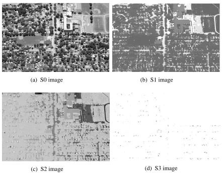
S [S0 S1 S2 S3]T (3-1) S0 is the total intensity image.
32 2 2 2 1 2
0 S S S
S (3-2) S1, S2 and S3 images describe the linear polarization, orientation and circular polarization content
of light in the scene respectively. These Stokes images can be calculated using the intensity
where I(0o), I(45o), I(90o), and I(135o) are the measured intensity images acquired with a corresponding polarizer. I(Rcirc) and I(Lcirc) are the right-circular and left-circular polarization
respectively. S1 represents the difference of intensity between horizontal and vertical linearly
polarized components. S2 is the difference between 45o and 135o linearly polarized components.
S3 is the difference between the right circular and the left circular component. The Stokes
parameters are related by equation 3-2. Only three of them are independent. Fig. 3-1 shows the
four Stokes images of the green band of the second frame of DIRSIG data.
Based on the Stokes parameters, other geometric features have been derived and used to
[image:18.612.101.542.259.603.2]characterize and explore the polarization phenomenon, such as the angle of polarization and the Figure 3-1: Four Stokes parameter images of the second frame of DIRSIG data
(a) S0 image (b) S1 image
degree of polarization. The angle of polarization is calculated as in the equation below,
depending on S2 and S1.
tan ( ) 2 1 1 2 1 S S
AoP (3-4)
The degree of polarization is calculated as:
0 2 3 2 2 2 1 S S S S
DoP (3-5)
where DoP is between 0 and 1. According to the value of DoP, three conditions are classified:
randomly polarized (DoP= 0), completely polarized (DoP= 1) and partially polarized (0<DoP<1).
Compared with the other three Stokes parameters, S3 is typically small. So when performing
remote sensing of the Earth, S3 can be neglected. We can simplify equation 3-5 to Degree of
Linear Polarization (DoLP):
0 2 2 2 1 S S S DoLP
DoP (3-6)
Fig. 3-2 show the DoP and AoP images respectively, calculated using the Stokes parameter
images shown in Fig. 3-1.
0 0.1 0.2 0.3 0.4 0.5 -40 -30 -20 -10 0 10 20 30 40
Figure 3-2: Degree of Polarization image and Angle of Polarization image
3.2 Multispectral Imaging
Multispectral imaging is a three-dimensional data cube, which is generated using several
spectral vectors for each pixel. The spectral vectors range from the visible region (0.4-0.7μm) to
the infrared (0.7-1μm). Each channel of the data cube can be displayed as a grayscale image and
the combinations of two or three channels as a color image. If the blue, green and red channels
are extracted, a true-color picture can be displayed.
Multispectral imaging contains both spatial and spectral information. If all the pixels of a
single ground resolution cell are extracted and one plots the spectral values as a function of
wavelength, the spectral information for that ground resolution cell is obtained. If all the pixels
in the same spectral band are extracted, the intensity values show the spatial distribution of
reflectance of the scene for that particular wavelength (EI-Sabe at al., 2010). Multispectral
imaging has been widely used in the remote sensing field for detection and tracking.
3.3 DIRSIG Data Set
DIRSIG, a physics-based synthetic image simulation software package, has been developed
by RIT CIS researchers and scientists. It has the ability to produce imagery in a variety of
modalities, such as multi-spectral, hyper-spectral and spectropolarimetric imagery, which can be
used to test the performance of spatial and spectral image analysis algorithms. DIRSIG contains
a graphical user interface editor which has five major simulation components and additional
options (Brown, 2006). They are scene modeling, atmosphere condition modeling, imaging
platform modeling, platform motion modeling, data collection and options respectively, as
shown in Fig. 3-3. The details about these simulation components are not introduced in this
The DIRSIG data set is all nadir imagery in this project, and are formed by assuming a static
sensor mounted on an aerial platform pointing directly toward a target stare point. Pixel pitches
are simulated as x=y=17 [µm/pix] square for the 2640*1680 image array. The flying height H
is equal to 2417 [m] AGL and the focal length is 204 [mm]. Based on the focal length and flying
height, the scale factor (s) can be calculated:
5 3 10 4 . 8 ] [ 2417 ] [ 10
204
m m H f
s (3-7)
The ground sample distance (GSD) can be computed:
0.20[ ]
10 4 . 8 ] [ 10 17 5 6 m m s x GSD
GSDX Y
(3-8)
The detector array physical dimensions for an 2640*1680 pixel detector:
lx nxx2640[pix]17[m/ pix]44.88[mm] (3-9)
ly nyy1680[pix]17[m/pix]28.56[mm] (3-10)
The total ground scene dimensions:
534[ ]
10 4 . 8 ] [ 88 . 44 5 m mm s l l x
X (3-11)
Figure 3-3: Five major simulation components plus Options inDIRSIG GUI
340[ ] 10 4 . 8 ] [ 56 . 28 5 m mm s l
lY y
(3-12)
The total field of view of the sensor is computed using the trigonometric relationship between
the focal length and the detector array dimensions.
x o o
x x mm mm f l HFOV
FOV ) 2 6.277 12.56
] [ 204 2 ] [ 88 . 44 ( tan 2 ) 2 ( tan 2
2 1 1
(3-13)
y y y o o
mm mm f
l HFOV
FOV ) 2 4.004 8
] [ 204 2 ] [ 56 . 28 ( tan 2 ) 2 ( tan 2
2 1 1
(3-14)
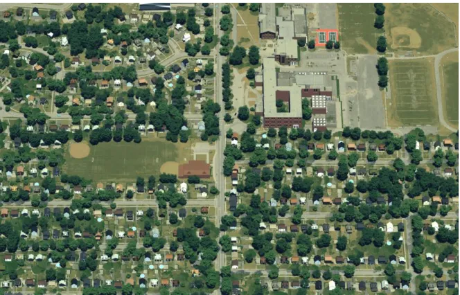
Each frame of this data set has 6 bands. The spectral range is 0.45 to 0.95 [um], with an
interval of 0.1 um. Further, polarized imagery includes four Stokes parameters corresponding to
each spectral band as simulated as well. Therefore, one frame of data has a total of 24 high
resolution images. There are 30 sequential frames data for this project to track vehicles. The
RGB bands (9th, 5th, 1st) of each frame can be extracted and adjusted for display together, as
[image:22.612.141.473.434.647.2]shown below in Fig. 3-4.
Different vehicles were simulated in DIRSIG with different vehicle paint. There are a total
of 21 vehicles in this project. Two of them are shown in the figures below.
There is no noise in the generated DIRSIG data sets. To see how the noise affects the
detection and tracking methods, a zero-mean Gaussian noise is added into data. The variance of
Gaussian noise is calculated using the following equation:
2 ( )2 SNR
(3-15)
where μ is the mean of intensity value of image, SNR is signal to noise ratio. Suppose SNR is
equal to 30 for the DIRSIG data with trees, the mean is calculated for each image in a frame.
Then using equation 3-15, the variance of each image is calculated. Final, Gaussian noise is
added into each image.
3.4 MAPPS Data Set
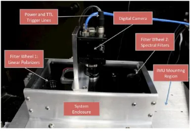
The MAPPS instrument can produce multi-spectral polarimetric imagery of scenes for use in
algorithm development and phenomenology studies. The main components of MAPPS consist of
a digital camera, two filter wheels, system enclosure and so on, as shown in Fig. 3-6. The first
filter wheel contains a set of linear polarizers, each oriented with their transmission axes rotated
relative to each other. The second filter wheel contains a set of spectral bandpass filters and can Figure 3-5: RGB image of vehicles simulated in the
allow for up to 10 different spectral bands to be collected. As each spectral filter and the linear
polarizer is rotated, spectral Stokes imagery can be collected (Bartlett et al., 2011).
When collecting the data set, the airplane flies at 4000 meters, the focal length of the digital
camera is 35mm and the pixel pitch is 3.45 um. According to Equation 3-8 and 3-7, the scale
factor s and the ground sample distance can be calculated respectively:
The detector array physical dimensions for an 2456*2058 pixel detector:
lx nxx2456[pix]3.45[m/ pix]8.47[mm] (3-18)
ly nyy2058[pix]3.45[m/ pix]7.1[mm] (3-19)
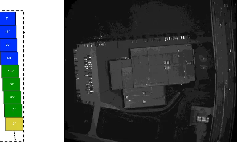
Only six spectral bands are chosen among the ten spectral filter set: blue (475nm), green
(550nm), yellow (607nm), red (655nm), rededge (716nm) and NIR2 (809nm). The polarization
filter set consists of four linear polarizers which allow generating four polarization images
[image:24.612.212.405.128.260.2]corresponding to the angle 0o, 45o, 90o, and 135o respectively. This data set has 24 frames since Figure 3-6: Illustration of the MAPPS system (From Bartlett et al., 2011)
6 3 10 75 . 8 ] [ 4000 ] [ 10
35
m m H f s ] [ 394 . 0 10 75 . 8 ] [ 10 45 . 3 6 6 m m s x X GSD X
GSDX Y
each spectral band consists of four polarizer images. Each frame is a one band one polarization
high resolution panchromatic image with dimensions of 2456*2058. Since each frame is
obtained from the sensor at a different time as the plane moves forward, image registration is
necessary to obtain accurate registered imagery. Fig. 3-7 (a) illustrates the sequence of MAPPS
data and (b) is the first frame image (blue band at 0o polarization).
3.5 Image Registration
Image registration is the process of overlaying images of the same scene taken at different
times, from different viewpoints, or different sensors. One of the images is referred to the base
image and the second image is referred as the sensed image. There are many ways to do image
registration, including frequency domain methods and spatial domain methods. Frequency
domain methods register the image in the transform domain (Persons et al., 2002). Spatial
[image:25.612.153.539.211.447.2]methods register the image in the image domain, matching intensity patterns or features in Figure 3-7: Illustration of sequence images MAPPS system and the first frame image
images (Goshtasby, 2005). In this project, the image registration is done in the spatial domain.
Image registration is described in the following.
Assume x and y are the coordinates of the base image and x' and y' are the coordinates of the
same ground location in the sensed image, the mapping function connecting to these two
coordinates is: ) , ( ' ) , ( ' y x g y y x f x (3-20)
f and g are high order polynomial mapping functions. Since the images needing registration in
this project only have translation and rotation, the mapping function can be simplified as:
y b x b b y y a x a a x 2 1 0 2 1 0 ' ' (3-21)
The mapping function coefficients are calculated using control points X and Y:
y T T x T T Y X X X b Y X X X a 1 1 ) ( ) ( (3-22) where T n n y y y y x x x x X 3 2 1 3 2 1 1 1 1 1 ' ' 2 ' 1 n x x x x Y ' ' 2 ' 1 n y y y y Y
Here T is the transpose and n is the number of control points. After obtaining the coefficients of
the mapping function, the image is finally registered with the process of geometric
transformation. To obtain the control points, the scale-invariant feature transform (SIFT) (Lowe,
2004) is used to match the features between the base image and the sensed image. The
coefficients of the mapping function can be calculated using the matched pairs. But the
calculated coefficients are not accurate because not all the matched pairs are right. Therefore, an
robustly estimate the coefficients of the affine transformation for image registration. These
algorithms are described further below.
3.5.1 Scale-Invariant Feature Transform (SIFT)
SIFT, proposed by David G. Lowe in 1999, is an algorithm to extract and identify a large
number of features (Lowe, 1999). Further, the method allows the descriptors to be reliably
matched using a large database of features. To generate the set of image features, SIFT needs
four major steps: scale-space extrema detection, keypoint localization, orientation assignment
and keypoint descriptor respectively.
The first step is to detect interest points for SIFT features, which correspond to local
extrema in the scale-space (Lowe, 1999). The scale space of an image can be defined as a
function, L(x,y,σ), that is the convolution of a variable-scale Gaussian with the input image. This
is the process to simulate the multiple scale property of the image.
) , ( * ) , , ( ) , ,
(x y G x y I x y
L (3-23)
Here I(x,y) is the input image and (2 2)/2 2
2
2 1 ) , ,
(
x y
e y
x
G is the Gaussian function using 2.
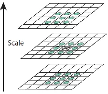
Lowe proposed the concept that using scale-space extrema in the difference-of Gaussian
(DoG) function convolved with the image to detect stable key-point locations in the scale space.
They can be computed from the difference of two nearby scales. The equation is shown below:
D(x,y,)(G(x,y,k)G(x,y,))*I(x,y)L(x,y,k)L(x,y,) (3-24) The initial image is incrementally convolved with Gaussians to produce images that differ by a
images (right side of the Fig. 3-8). After each octave, the Gaussian image is downsampled by a
factor of 2 and the process is repeated.
In the DoG image, each pixel, such as the one marked X in Fig. 3-9, is compared to its eight
neighbors in the current image and nine neighbors in the scale above and below to decide the
local maxima and minima of D(x,y,σ), as shown in Fig. 3-9. If the pixel is a local maximum or
minimum, it is selected as a candidate keypoint.
The next step is to perform accurate keypoint localization. Points with low contrast and
[image:28.612.252.361.513.608.2]those that are poorly localized along an edge are rejected. Brown has developed a method to Figure 3-8: Illustration of the formation process of scale space and DoG
(From Lowe, 2004)
Figure 3-9: Illustration of the process of finding a candidate keypoint (From Lowe, 2004)
Difference of Gaussian Scale
(next octave)
perform keypoint localization (Brown et al., 2002). The method uses the Taylor expansion of
scale-space function and shifts so that the origin is at the sample point.
x x D x x x D D x D T T 2 2 2 1 ) (
(3-25)
Where x=(x,y,σ)T is the offset from this sample point. By taking the derivation of this function
with respect to x and setting it to zero, the location of the extremum can be expressed as:
x D x D x 2 1 2 (3-26)
By substituting Equation 3-26 to Equation 3-25, the function value at the extremum, ( )
x
D , can be
obtained: x x D D x D T 2 1 )
( (3-27)
All extrema with a value of ( )
x
D less than 0.03 are discarded.
To assign the orientation, a gradient orientation histogram is calculated in the neighborhood
of the keypoint. The peak in the histogram corresponds to the dominant direction. This process
is to test the rotation-invariant property of the keypoint.
The final step is to compute the keypoint descriptor. As is shown in Fig. 3-10 (a), a 16x16
window is regarded as the neighborhood of the keypoint. Each pixel has the gradient orientation
and magnitude, which is indicated as the direction and length of the arrow respectively. In each
4x4 small window, eight orientation histograms are computed and accumulated. A descriptor is
formed. The keypoint has 4x4 descriptor array and each contains 8 bin histograms. So a SIFT
Euclidean distance was used to match the keypoints in the two images. First, the distances
between one keypoint in the first image and each keypoint in the second image were calculated.
Then in the second image, two points with the first nearest and second nearest distance were
selected and the quotient (first nearest distance divided by the second nearest distance) was
calculated. If the result was less than the specified threshold that is 0.6 in the Lowe's paper, the
keypoint in the second image with the nearest distance was the matched point. Finally, repeat
this process for all keypoints to find out all match pairs.
3.5.2 Random Sample Consensus (RANSAC)
RANSAC, a randomized estimator, was introduced by Fischler and Bolles (Fischler at al.,
1981). This algorithm is commonly used to estimate the parameters of a model, using data that
may be contaminated by outliers. RANSAC estimates a relation that fits the data, while
simultaneously classifying data into inliers (points that fit the relation) and outliers (points that
do not fit the relation). Due to its ability to tolerate a large fraction of outliers, this algorithm has
been widely applied to estimation problems in computer vision, such as feature matching and
registration.
RANSAC operates in a hypothesize-and-verify process. First randomly select the samples
from the input data set. The model parameters are computed using the sample data. The size of Figure 3-10: Illustration of the computation of keypoint
descriptor (From Jonas Hurreimann)
the sample depends on the model. For example, to calculate the affine transform parameters in
image registration, three points are needed. In the next step, the quality of the model is evaluated
on the full data set by calculating the error for each point. Then determine how many points from
the set of all points fit within a predefined tolerance error ϵ. If the number of the inliers exceeds a
predefined threshold τ, re-estimate the model parameters using all the identified inliers and
terminate. If not, this hypothesize-and-verify loop is repeated until the criterion is met.
Two thresholds are used in the RANSAC operation. One is the error for each point to
determine whether or not it agrees with the model. This threshold is equal to 5 in this thesis.
Another is the number of inliers. This threshold is half of matched pairs that are different frame
by frame. Take the frame 16 as an example, there are 55 matched pairs as listed in Fig. 3-11(a),
so the threshold for this frame is 27. The advantage of RANSAC is its ability to do robust
estimation of the model parameters, but it can only estimate one model for a particular data set.
RANSAC may fail when more than one model exist in the data set.
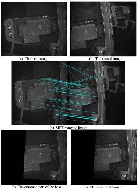
3.5.3 Registration Result
For the MAPPS data, the first frame image is regarded as the base image; all other images
are registered based on the first image. Take the frame 16 as the example; it is registered based
on the first frame. In Fig. 3-11, (a) is the first base image, (b) is the sensed image (the sixteenth
frame), (c) shows the matched pairs between (a) and (b) using SIFT, (d) is the common part of
(d) The common part of the base
image with the sensed image
[image:32.612.88.528.69.668.2](e) The registered image
Figure 3-11: Illustration of image registration for MAPPS data (c) SIFT matched image
Not all the matched pairs are correct in Fig. 3-11 (c). When matching the keypoints in two
images, the specified threshold ( equal to 0.6 in Lowe's paper) is a criterion to decide whether
two keypoints are the matched pair or not. The detailed procedure is discussed at the end of
section 3.5.1. If the threshold is decreased, the number of matched pairs is less. Otherwise, the
number of matched pairs is more. The number of wrongly matched pairs is also increased.
However, these wrongly matched pairs do not affect registration result, because RANSAC is
used to robustly classify matched pairs into inliers and outliers points.
To evaluate the result of image registration, the Peak Signal to Noise Ratio (PSNR) is used
to quantitatively analyze. The PSNR term describes the similarity between two images and its
unit is decibel (dB). The equation is defined as following:
MSE PSNR
n 1)2
2 ( log
10
Where n is the number of bits. The mean–squared error (MSE) represents the average squared
difference between the digital counts from two compared images. The equation is defined as
below:
r c N
i N
j
ij ij
N N
f f MSE
C r
1 1
2
) (
Where fijand fijare the digital counts of the two compared images and Nc and Nrare the number
of columns and rows in both images.
Generally speaking, the greater the value PSNR, the smaller the difference between images,
the more similar two images, and the better the quality of the registered image; contrarily, the
smaller value, the greater difference is, two images are more different and the quality is poorer.
Generally, the registered image has the great similarity with the base image when PSNR is larger (3-28)
than 30. PSNR and MSE between image (e) and (d) are 34.2 and 24.7 respectively, which
4 Methods
For tracking vehicles it is necessary to detect the vehicles first, because we do not know the
ground location for each vehicle. In this chapter, the target detection methods and the tracking
algorithms are described.
4.1
Detection
Three target detection methods are used in this thesis. Local adaptive threshold method
(Shafait et al., 2008) is applied to the MAPPS data set. Two other methods, RX (Reed et al.,
1990) and change detection (Radke et al., 2005) are combined to detect the vehicles in the
DIRSIG data set.
4.1.1
Local Adaptive Threshold
To segment the foreground objects, a threshold is commonly used. Pixels with intensity
values above a threshold are considered as the foreground, and all the remaining pixels are the
background.
otherwise
y x t y x g if y
x D
0
) , ( ) , ( 1
) ,
( (4-1)
For the conventional threshold methods, the threshold t(x,y) is constant across the whole
image, while the local adaptive threshold method varies the threshold dynamically across the
whole image. For each pixel in the image, a threshold is calculated. The way to find the local
threshold depends on the intensity values of the local neighborhood of each pixel. The mean or
the median of the local neighborhood can be regarded as the threshold. The size of the
neighborhood window has to be large enough to cover both foreground and background pixels;
otherwise a poor threshold is chosen. In this thesis, the window size is about 60*60 pixels,
When the mean or median value lies between the intensity values of foreground and
background, they are separated easily. If the range of intensity values within a local
neighborhood is very small, the mean of the local area is not suitable as a threshold, because its
mean is close to the value of the center pixel. Finally, the threshold employed is not the mean,
but (mean-C), where C is a constant value and can be negative or positive. All pixels in a
uniform neighborhood are set to the background.
4.1.2
RX Detector
The RX detector (RXD) was developed by Reed and Yu to detect targets whose signatures
are distinct from their background. This method is commonly used to detect the small targets for
multi-spectral and hyperspectral images (Bartlet et al., 2011). The main idea of RXD is to use the
sample covariance matrix to take into account the sample spectral correlation; it performs as the
Mahalanobis distance.
) ( )
( )
(x x m 1 x m
R T (4-2)
where x is the pixel spectral vector, m is the mean spectral vector and is the sample
covariance matrix of the image. Suppose that L is the number of spectral bands, then x is a L*1
column vector and is a L*L matrix. The equation illustrates that the RXD algorithm
computes the Mahalanobis distance from each pixel to the spectral distribution of the global
image. A large R(x) value corresponds to points that may be anomalous. Since the images
produced by the RXD are generally grayscale, a threshold is needed to segment targets from the
image background.
4.1.3
Change Detection
Moving target detection and segmentation can be achieved using change detection.
equation 4-3, It(x) and It-1(x) represent the current frame and the adjacent previous frame
respectively. To threshold the difference image D(x), the change mask B(x) is generated
according to the equation 4-4.
D(x)It(x)It1(x) (4-3)
otherwise x D if x B 0 ) ( 1 )
( (4-4)
The threshold τ is chosen empirically. In this thesis, τ is mostly equal to 0.001 with the units of
[W/cm2/sr/μm], because DIRSIG typically generates spectral radiance imagery.
4.1.4
Combined Method
Both RX detection and change detection have shortcomings. For RX detection, non-moving
man-made objects, such as buildings, may be detected as an anomaly. Therefore, some false
alarms are produced using RX detection. For change detection, not all the background is stable
from one frame to next frame, so some pixels are mistakenly considered as the foreground object.
To overcome the disadvantages of both methods, the two binary images obtained from RX and
change detection can be multiplied at the pixel level with the objective of suppressing false
detections not present in both methods. This combined method obtains a good result because
only anomalies in both binary images are likely to be selected as detections. Fig. 4-1 shows the
process of the combined detection method. Frame t and frame t-1 are the adjacent frames at time
t and t-1 respectively.
4.2 Motion Tracking
Motion tracking depends on measurements of the locations and velocity to track vehicles.
Fig. 4-2 is the flow chart of motion tracking used in this thesis. Assume there are N vehicles in
the frame t, each vehicle is initialized with Kalman filter, and then predict the location in the next
frame. Depending on the predicted location and the measurements, GNN (Global Nearest
Neighbor) data association is applied to assign the measurements to the existing tracks. The
measurements that are not assigned are regarded as new vehicles and initialized as new tracks.
Finally, all the trackers predict the location in the next frame. In the following section, the
Kalman filter and GNN algorithm are introduced.
4.2.1 Kalman Filter
A Kalman filter (Maybeck, 1979) is used to estimate the state of a linear system. The state
can refer to any measurable quantity, such as an object’s location or velocity. The Kalman filter
is a recursive two-stage filter. At each iteration, it is composed of a predict phase and an update
phase.
The predict phase predicts the current location of the moving object based on the previous
observation. We consider a tracking system where xk is the state vector which represents the
Figure 4-2: The flow chart of motion tracking Gating
N vehicles
Associa tion
i
New trackers frame t
Update
frame t+2
predict frame t+1
dynamic behavior of the object, where subscript k indicates the discrete time. The equations for
the predict phase are as following:
the system estimate:
1
k k Ax
x (4-5)
the state prediction covariance:
Q A P A
P T
k
k 1 (4-6)
where, A is the state transition matrix, xk and xk-1 represents the state at time k and k-1
respectively, Q is the noise covariance of the system. P is the predicted estimate covariance.
The update phase involves other system information, an observation as well as estimate
calculations. When an observation zk is made, the residual of that measurement is calculated as:
k k
k z H x
y (4-7)
H is the measurement matrix.
The optimal Kalman gain Kk is computed:
1 )
(
PH HPH R
Kk k k T (4-8)
Where, R is the observation noise covariance. Based on the above equation, the state update and
the covariance update are computed as below:
k k k
k x K y
x 1 (4-9)
k k
k I K H P
P1 ( ) (4-10)
After the xk+1 and Pk+1 is computed, they are used recursively to predict a new estimate. This
recursive behavior of estimating the states is one of the highlights of the Kalman filter.
The system models of Kalman filters depend on a case by case analysis. The dimension of
spatial size and so on. The system models of the Kalman filters for the two data sets considered
here are different. The vehicles in the MAPPS data set move in two directions, nearly parallel.
So the state vector x0 is initialized using the top-left position of the tracking window (rectangular)
as shown in Fig. 4-3(a), and velocity. The size of the tracking window is the same for all vehicles
with the width 30 and height 50 pixels. For velocity, one method to initialize it is to use the
difference between two positions from the first two consecutive frames. But it is convenient and
effective to initialize with zero velocity and a large state covariance. The initialization of each
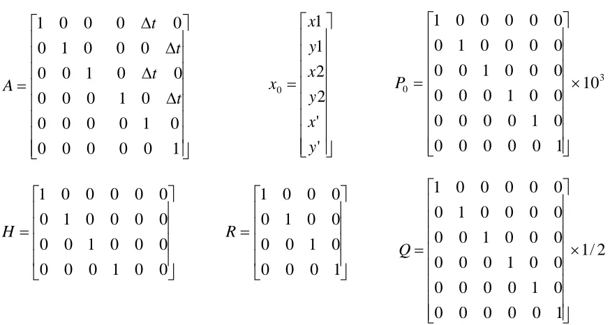
parameter for MAPPS data is listed below respectively.
A is the state transition matrix, P0is the state covariance and x0 is the state vector. tis the time
interval between two adjacent frames and it is equal to 1 in MAPPS data. The measurement
transition matrix H, the measurement noise covariance R and process noise covariance Q are
listed below:
For the DIRSIG data set, the vehicles move in all directions. It is improper to set the size of
tracking window of all the vehicles same. So the state vector used in DIRSIG data set is different
from the one in the MAPPS data set. The state vector is six dimensional vector with the top-left
and bottom-right locations of the tracking window and the velocity x' and y', as shown in Fig.
4- 1 0 0 0 0 1 0 0 0 1 0 0 0 1 t t A ' ' 0 y x y x x 4 0 10 1 0 0 0 0 1 0 0 0 0 1 0 0 0 0 1 P 0 0 1 0 0 0 0 1 H 1 0 0 1
R 1/2
3(b). Other parameters are also correspondingly changed. The total of six parameters are
initialized as below:
here, t is equal to 5 and x0 is initialized with the detected location and zero velocity.
4.2.2 Global Nearest Neighbor Approach
In a multiple target tracking (MTT) system, data association is very important because the
received measurements may not all arise from the real targets. Some of them may be from false
alarms. Therefore, there always exist ambiguities in the association between the previous known
1 0 0 0 0 0 0 1 0 0 0 0 0 1 0 0 0 0 0 1 0 0 0 0 0 1 0 0 0 0 0 1 t t t t A ' ' 2 2 1 1 0 y x y x y x
x 0 103
[image:41.612.94.531.121.354.2]1 0 0 0 0 0 0 1 0 0 0 0 0 0 1 0 0 0 0 0 0 1 0 0 0 0 0 0 1 0 0 0 0 0 0 1 P 0 0 1 0 0 0 0 0 0 1 0 0 0 0 0 0 1 0 0 0 0 0 0 1 H 1 0 0 0 0 1 0 0 0 0 1 0 0 0 0 1 R 2 / 1 1 0 0 0 0 0 0 1 0 0 0 0 0 0 1 0 0 0 0 0 0 1 0 0 0 0 0 0 1 0 0 0 0 0 0 1 Q Road 50 30 (x, y) Road (x1, y1) (x2, y2) (x1, y1) (x2, y2)
Figure 4-3: Illustration of initiation of Kalman Filter (red point indicates the initial position)
targets and measurements. Assigning a wrong measurement to an existing track often results in a
lost track or wrong track.
Many data association methods are used in MTT systems, ranging from simple methods to
complex ones, such as multiple hypotheses tracking (MHT) (Reid, 1979). The simple method,
such as suboptimal nearest neighbor (Farina et al., 1985), can be easily implemented in MTT
system, but its performance is degraded in a cluttered environment. The MHT method provides
improved performance, but it is difficult to implement and a large number of hypothesis may be
maintained. Global Nearest Neighbor method (Konstantinova et al., 2003) gives an optimal
solution. Before associating the observation to tracker, gating is implemented first.
4.2.2.1Gating
Gating (Blackman, 1986) is a coarse test for eliminating unlikely observation-to-track
pairings. A gate is formed around the predicted position of a Kalman filter. All measurements
within the gate are considered for updating this track. Actually, the measurement to update the
track depends on the data association. The measurements outside the gating may be false alarms
or newly appeared targets.
Using the Kalman filter, the state vector and the state covariance are predicted as in
equations 4-5 and 4-6 respectively. The predicted measurement is:
k k Hx
z' (4-11)
The residual vector between measured and predicted quantities is:
) ( ' ) ( ) (
'
k z k z k
zij j i (4-12)
zj is the j-th measurement, zi is the i-th track predicted vector. The residual covariance matrix is
computed:
R H HP k
A validation region is defined as :
where G is the gate threshold. The
measurements within the gate or on the boundary of the gate are the validated measurements.
4.2.2.2Association
Data association takes the output of the gating algorithm and makes the final
measurement-to-track association (Bogler, 1989). When a single measurement lies in the gate of a single track,
an assignment can be made immediately. But the conflict situation will arise when multiple
measurements falls within a single gate or when a single measurement falls within the gates of
several tracks. Fig. 4-4 illustrates the conflict situation. In the three predicted locations (P1, P2
and P3) for three trackers, corresponding gates are formed. Three measurements (O1, O2 and O3)
fall in these gates. But the measurement O2 falls in the intersection of the gates of the three
trackers. By calculating the distance from each measurement to each predicted location, the
GNN method can decide which measurement should update which tracker.
We assume there exist a set of n tracks and m measurements at the time index k, with m not
necessary equal to n. A validation gate is defined by equation 4-14. The choice of G has to
ensure that the correct measurements will lie within the gate. We define the cost matrix C
(Konstantinova et al., 2003) for the assignment problem. The entries in matrix C are determined
depending on equation 4-15. If measurement j is not in the gate of track i, the entry is set to 100;
G z S z
[image:43.612.238.405.438.540.2]dij2 ij'T i1 ij' (4-14)
otherwise, the entry is set to the squared Mahalanobis distance from the measurement j to the
track i.
n c c c c c c c c c c c c c c c C j nm n n n n m m ij 2 1 4 3 2 1 2 24 23 22 21 1 14 13 12 11 i i track of gate the in is j t measuremen if d i track of gate the in not is j t measuremen if C ij ij 2 100 (4-15)
The desired solution of the cost matrix is the one that minimizes the summed total distance.
We use the Munkres algorithm (Munkres, 1957 and Bourgeois et al., 1971) to solve the
assignment problem. But due to missed detections, it is possible that some tracks are associated
with a measurement that is not in the gate of the track. So it is necessary to check the values of
matrix C.
4.2.2.3 Munkres Algorithm
The Munkres method is an optimal method to solve the assignment problem. The goal of
this method is to assign jobs to workers so as to minimize the total cost. This method has 6 steps:
Step 1: Create an N*M cost matrix in which each element represents the cost of assigning
one of N workers to one of M jobs. The matrix can be rectangular or square.
K=min(N,M).
Step 2: For each row, find the row minimum and subtract it from all entries on that row.
Step 3: For each column, find the column minimum and subtract it from all entries on that
column.
Step 4: Draw lines across rows and columns to cover all zeros using the minimum number of
Step 5: If the number of lines drawn is equal to K, the assignment is finished. If not, go to
step 6.
Step 6: Find the smallest entry which is not covered by the lines, subtract it from each entry
not covered by the lines, and add it to each entry which is covered by line. Then go
back step 4.
To easily understand this algorithm, an example is used. Suppose there are three vehicles
and three measurements, so K is equal to 3. In the cost matrix Cij, 1, 2 and 3 are the minimum of
each row respectively. Through step 2, the second matrix is obtained. 0, 1 and 2 are the
minimum of each column in the second matrix. Subtract the column minimum, and the third
matrix is formed. The minimum number of lines to cover all the zeros is 2, less than 3, so step 6
is implemented. In matrix four, 1 is the minimum entry that is not covered by the line.
Subtracting it from each entry not covered by the lines, the fifth matrix is formed. Now draw
lines again, three lines are needed to cover all zeros, so the assignment is finished. The
measurements 3, 2 and 1 are used to update tracker 1, tracker 2 and tracker 3 respectively.
3 1 0 1 0 0 0 0 0 3 1 0 1 0 0 0 0 0 4 2 0 2 1 0 0 0 0 4 2 0 2 1 0 0 0 0 6 3 0 4 2 0 2 1 0 9 6 3 6 4 2 3 2 1 ij C
4.3
Feature Matching
In a complex environment, motion tracking often fails when vehicles split or vehicles are
re-detected after missing detection. Motion tracking regards the detections that are not assigned
using Munkres Algorithm as the new ones. This case is not always true because they may be the
ones that existed before. Feature information, such as spectral measurements, can identify and
measurements j
distinguish the vehicles because different materials have different spectral information. So
spectral histogram based tracking (Nguyen et al., 2010 and Brown et al., 2006) is widely used for
object tracking.
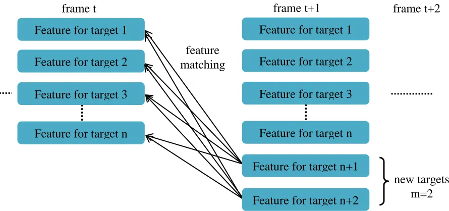
The process of spectral feature matching is shown in Fig. 4-5. Assume there are n targets in
the frame t and a rectangular target region identifies each target. The spectral feature in each
target region is extracted and a histogram is computed. In the next frame, m new targets appear
and the corresponding features are also extracted. The features of each new target are compared
with the features of prior frames to check whether the new appeared target is a new one or the
one existed before. If the minimum of compared results is above the threshold, this target is
regarded as the new target, otherwise, this target is marked as an existing target which has been
re-detected again.
The statistical measure, Bhattacharyya measure (Djouadi et al., 1990 and Kailath, 1967), is
used to calculate the similarity between histograms. The Bhattacharyya coefficient (p,p')
[image:46.612.84.529.377.586.2]measures the amount of relative closeness between two statistical samples: Figure 4-5: The illustration of feature matching
feature matching Feature for target 1
frame t
Feature for target 2
Feature for target 3
Feature for target n
new targets m=2 Feature for target 1
frame t+1
Feature for target 2
Feature for target 3
Feature for target n
Feature for target n+1
Feature for target n+2
Where p and q represent the spectral probability density function (spdf) of the reference object
and the candidate object respectively, each consisting of Nm bins with respective probability pu
and qu. N is the number of bands and m is the number of bins for each band.
The distance between two histograms is defined as:
When dBhatis equal to 1, it means the maximum mismatch happens; when dBhatis equal to zero,
it means two histograms have maximum match.
4.4 Feature Aided Tracking
Motion tracking regards all the detections that are not used to update trackers as new ones.
Actually, they are not always new ones. So motion-only tracking will assign the wrong track for
some targets. Adding features into tracking will solve this problem. Since the illumination may
slightly vary between frames, the histogram may be not same for each target in all frames. In this
thesis, the features of each target at each frame are stored in order to improve the matching
accuracy.
Each target has four properties, position, velocity, identification and feature. For the second
frame (this is the first tracking frame owing to use change detection), the position is initialized
using the detected result and the velocity is initialized to zero for each target. Also identification
is marked and features extracted for each target. Assume in frame t, there are n detected targets
and each one has been assigned a tracker. In the frame t+1, m targets are detected and the
corresponding features extracted. Depending on the GNN data association, some detections are
Nm
u
u uq p q
y p y
1
) ), ( ( )
(
) ( 1 )
(y y
dBhat
(4-16)
used to update the n trackers. The features of the remaining detections are compared with all the
features of prior frames to check whether they are the targets that existed before or new ones.
The Bhattacharyya distance is used to measure the similarity between features. If the minimum
Bhattacharyya distance among a group of distances is above the threshold, this target is a new
one; otherwise, it is corrected with the prior tracking ID. The threshold used in this thesis is
0.447, which means the similarity of features should be at least 80%. If there is no detection to
update one track in three-adjacent frames, this track is given up. Fig. 4-6 is the flow chart of the
feature-aided tracking algorithm.
predict GNN
N trackers &feature
table
measurements assigned to update the corresponding
trackers
feature matching
frame t
minimum >threshold
frame t+1
Measure- ments
i
trackers no measurements
to update
Is the third frame
give up
extract features of not assigned measurements
new one existed one
assign new tracker predict
No Yes
[image:48.612.69.543.297.653.2]Yes No
4.5 Metrics for Performance Evaluation
Performance evaluation metrics aim to quantitatively analyze the tracking performance
based on system results and ground truth data. In most cases, system results could differ from
ground truth because of possible errors. Comparing system results and ground truth, four
outcomes are possible. These are true positives, false positives, true negatives and false negatives.
In a tracking problem, true positives are typically named "correct tracks", false positives are
"false alarms", true negatives are ones that switch to other tracks and false negatives are "lost
tracks". Based on these four classifications, the metric, Multiple Object Tracking Accuracy
(MOTA), can be computed.
where mt, fpt and met are the number of misses, of false alarms and of ones that switch to other
tracks respectively at time t. gt is the ground truth for time t. The MOTA can be seen as
subtracting 3 error ratios from 1.
is the ratio of misses in the sequence, computed over the total number of objects present in
all frames. The ratio of false alarms and the ratio of mismatches are calculated as in the below
equation in a similar way.
) (
1 m fp me
MOTA (4-18)
t t
g m
m (4-19)
m
t t
g fp fp
t t
g me
me
(4-20)