Single to multiple target, multiple type visual tracking

(1)

SINGLE TO MULTIPLE TARGET,

MULTIPLE TYPE VISUAL

TRACKING

submitted by

Nathanael Lemessa Baisa

for the degree of

Doctor of Philosophy of the

Department of Electrical, Electronic and Computer Engineering

Heriot-Watt University

October, 2017

This copy of the thesis has been supplied on the condition that anyone who consults it is understood to recognise that its copyright rests with its author and that no quotation from the thesis and no information derived from it may

(2)

ABSTRACT

Visual tracking is a key task in applications such as intelligent surveillance, human-computer interaction (HCI), human-robot interaction (HRI), augmented reality (AR), driver assistance systems, and medical applications. In this thesis, we make three main novel contributions for target tracking in video sequences.

First, we develop a long-term model-free single target tracking by learning discrimi-native correlation filters and an online classifier that can track a target of interest in both sparse and crowded scenes. In this case, we learn two different correlation filters, translation and scale correlation filters, using different visual features. We also include a re-detection module that can re-initialize the tracker in case of tracking failures due to long-term occlusions.

Second, a multiple target, multiple type filtering algorithm is developed using Random Finite Set (RFS) theory. In particular, we extend the standard Probability Hypothesis Density (PHD) filter for multiple type of targets, each with distinct detection proper-ties, to develop multiple target, multiple type filtering, N-type PHD filter, whereN ≥2, for handling confusions that can occur among target types at the measurements level. This method takes into account not only background false positives (clutter), but also confusions between target detections, which are in general different in character from background clutter. Then, under the assumptions of Gaussianity and linearity, we extend Gaussian mixture (GM) implementation of the standard PHD filter for the proposed N-type PHD filter termed as N-type GM-PHD filter.

Third, we apply this N-type GM-PHD filter to real video sequences by integrating object detectors’ information into this filter for two scenarios. In the first scenario, a tri-GM-PHD filter is applied to real video sequences containing three types of multiple targets in the same scene, two football teams and a referee, using separate but confused detections. In the second scenario, we use a dual GM-PHD filter for tracking pedestri-ans and vehicles in the same scene handling their detectors’ confusions. For both cases, Munkres’s variant of the Hungarian assignment algorithm is used to associate tracked target identities between frames.

We make extensive evaluations of these developed algorithms and find out that our methods outperform their corresponding state-of-the-art approaches by a large margin.

(3)

(4)

ACKNOWLEDGMENT

First and foremost, I would like to thank GOD for providing me the chance to pursue my dreams of following this PhD program. Next my deepest gratitude goes to UK En-gineering and Physical Sciences Research Council (EPSRC), James Watt Scholarship and all members of the Heriot-Watt University for giving me the opportunity to have these wonderful PhD program in my life. A very special gratitude goes to my super-visor, Prof. Andrew Wallace, who has supported me throughout my PhD program. I appreciate his technical support, and continuous follow up of my progress in designing, implementing as well as writing up my PhD dissertation. I also would like to thank Dr. Daniel Clark for his valuable suggestions and technical support in area of the technique I am using in this dissertation. I must also acknowledge Dr. Deepayan Bhowmik for his ideas and comments he provided me to adapt to the work environment and technical support. My appreciation also goes to all computer vision lab members of Heriot-Watt University for showing their hospitable behaviour of welcoming international students.

Lastly but not least, I would like to thank my family without their love and long sup-port, I would not be here to fulfil my dream. In particular, I must acknowledge my mother, Dashi Merera, without her love and encouragement, I would not have achieved my dreams.

Nathanael Lemessa Baisa October, 2017

(5)

Please note this form should be bound into the subm itted thesis.

Academic Registry/Version (1) August 2016

ACADEMIC REGISTRY

Research Thesis Submission

Name: Nathanael Lemessa Baisa School: School of Engineering and Physical Sciences Version: (i.e. First,

Resubmission, Final) Final Degree Sought: Doctor of Philosopy (PhD) Electrical Engineering

Declaration

In accordance with the appropriate regulations I hereby submit my thesis and I declare that: 1) the thesis embodies the results of my own work and has been composed by myself

2) where appropriate, I have made acknowledgement of the work of others and have made reference to work carried out in collaboration with other persons

3) the thesis is the correct version of the thesis for submission and is the same version as any electronic versions submitted*.

4) my thesis for the award referred to, deposited in the Heriot-Watt University Library, should be made available for loan or photocopying and be available via the Institutional Repository, subject to such conditions as the Librarian may require

5) I understand that as a student of the University I am required to abide by the Regulations of the University and to conform to its discipline.

6) I confirm that the thesis has been verified against plagiarism via an approved plagiarism detection application e.g. Turnitin.

* Please note that it is the responsibility of the candidate to ensure that the correct version of the thesis is submitted. Signature of

Candidate:

Date:

Submission

Submitted By (name in capitals): NATHANAEL LEMESSA BAISA

Signature of Individual Submitting:

Date Submitted:

For Completion in the Student Service Centre (SSC)

Received in the SSC by (name in capitals):

Method of Submission

(Handed in to SSC; posted through internal/external mail):

E-thesis Submitted (mandatory for final theses)

(6)

List of Figures

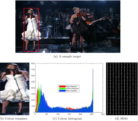
2.1 Examples of target representations: (a) a sample target (rectangular red bound-ing box) and correspondbound-ing (b) colour template and (c) colour histogram (Y-axis is the number of pixels in the image at each intensity value along X-(Y-axis) and (d) HOG feature visualization.. . . 10

2.2 One-stream Alex Net [1]. The network’s input is 227×227×3 = 154, 587-dimensional, and the number of neurons in the network’s remaining lay-ers is given by 290,400 - 186,624 - 64,896 - 64,896 - 43,264 - 4096 - 4096 - 1000. . . 14

2.3 Data association problem: two validated measurements (green boxes) are located in the validation region (grey area) centred on the predicted measurement (red triangle) [2]. . . 31

2.4 Single target to multi-target extension using RFS theory. The black arrows show the extension of single target tracking in which states and observations are represented using random vectors to multi-target tracking though FISST framework in which states and observations are represented using random finite sets. . . 39

2.5 FISST framework. . . 39

2.6 Probability hypothesis densities (PHDs) in two consecutive time steps [3]. . . . 39

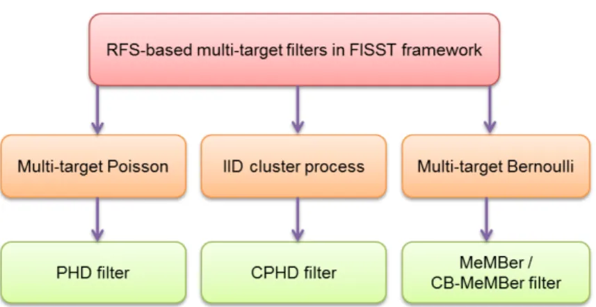
2.7 RFS-based multi-target filters in the FISST framework. . . 41

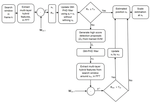
3.1 The flowchart of the proposed algorithm. It consists of three main parts: trans-lation estimation, re-detection and scale estimation. . . 51

(12)

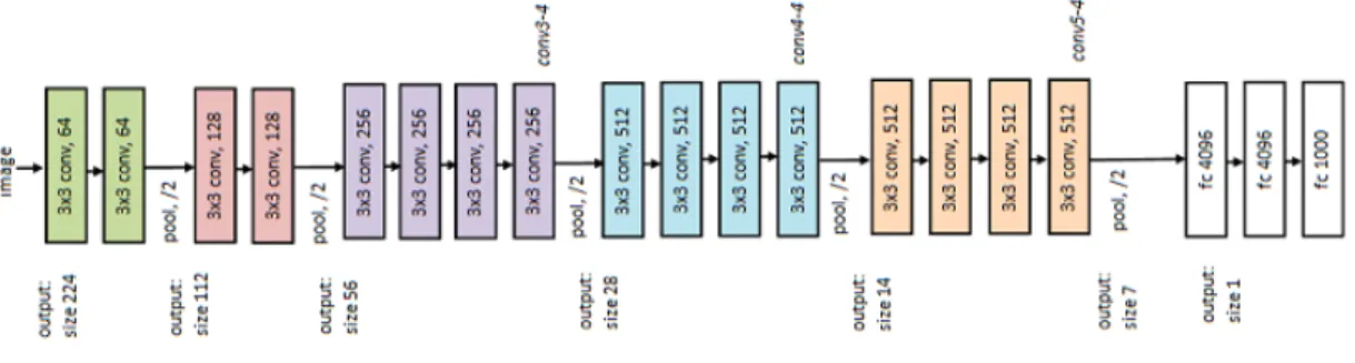
3.2 VGG-Net 19 [4]. . . 63

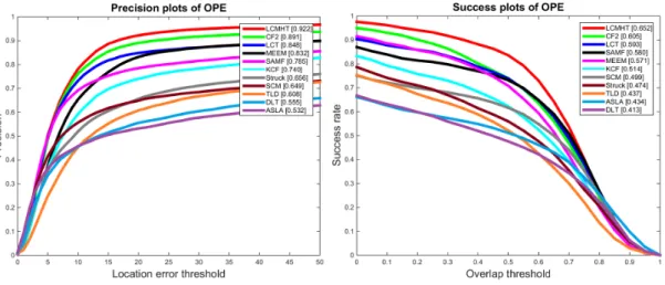
3.3 Distance precision (left) and overlap success (right) plots on OOTB using one-pass evaluation (OPE). The legend for distance precision contains threshold scores at 20 pixels while the legend for overlap success contains the AUC score of each tracker; the larger, the better. . . 65

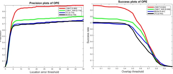
3.4 Distance precision (left) and overlap success (right) plots on OOTB using one-pass evaluation (OPE). The legend for distance precision contains threshold scores at 20 pixels while the legend for overlap success contains the AUC score of each tracker; the larger, the better. The performances of our algorithm (LCMHT) and its version without a re-detection module (LCMHT WtR) are shown. . . 65

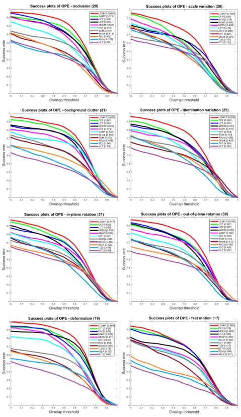
3.5 Success plots on OOTB using one-pass evaluation (OPE) for 8 challenge at-tributes: occlusion, scale variation, background clutter, illumination variation, in-plane rotation, out-of-plane rotation, deformation, and fast motion. The legend contains the AUC score of each tracker; the larger, the better. . . 67

3.6 Qualitative results of our proposed LCMHT algorithm, CF2 [5], MEEM [6], LCT [7] and KCF [8] on some challenging sequences of OOTB (Fleetface, Singer1, Freeman4, and Walking2 from left column to right column, respec-tively). . . 68

3.7 Distance precision (left) and overlap success (right) plots on PETS data sets using one-pass evaluation (OPE). The legend for distance precision contains threshold scores at 20 pixels while the legend for overlap success contains the AUC score of each tracker; the larger, the better. . . 69

3.8 Distance precision (left) and overlap success (right) plots on PETS data sets using one-pass evaluation (OPE). The legend for distance precision contains threshold scores at 20 pixels while the legend for overlap success contains the AUC score of each tracker; the larger, the better. The performances of our algo-rithm (LCMHT) and its version without a re-detection module (LCMHT WtR) are shown. . . 70

3.9 Qualitative results of our proposed algorithm LCMHT, CF2 [5], MEEM [6], LCT [7] and KCF [8] on PETS 2009 medium density (left column) and dense (right column) data sets. . . 72

(13)

3.10 Qualitative results of our proposed LCMHT algorithm, CF2 [5], MEEM [6], LCT [7] and KCF [8] on PETS 2009 medium density (left, frame 78) and dense (right, frame 85) data sets, just after occlusion by cropping and enlarging. . . 73

4.1 A sensor setting for our approach. The sensor is equipped with many detectors for each type of multiple targets in which case one detector can also detect other than its own target type resulting in separate but confused measurements which are filtered and discriminated by our approach. . . 75

4.2 Confusions between four target types (T1, T2, T3 and T4) at the detection stage from detectors 1, 2, 3 and 4. . . 92

4.3 Simulated ground truth (red, black, yellow and magenta for target type 1, 2, 3 and 4, respectively) and position estimates from four independent GM-PHD filters (blue circles, green triangles, cyan asterisks and black circles for target type 1, 2, 3 and 4, respectively) usingp12,D=p13,D=p14,D =p21,D =p23,D= p24,D=p31,D=p32,D =p34,D =p41,D=p42,D=p43,D = 0.3. . . 94

4.4 Simulated ground truth (red, black, yellow and magenta for target type 1, 2, 3 and 4, respectively) and position estimates from quad GM-PHD filter (blue circles, green triangles, cyan asterisks and black circles for target type 1, 2, 3 and 4, respectively) using p12,D =p13,D =p14,D =p21,D =p23,D =p24,D = p31,D=p32,D=p34,D =p41,D =p42,D=p43,D= 0.3. . . 95

4.5 Simulated ground truth (red, black, yellow and magenta for target type 1, 2, 3 and 4, respectively) and position estimates from four independent GM-PHD filters (blue circles, green triangles, cyan asterisks and black circles for target type 1, 2, 3 and 4, respectively) usingp12,D=p13,D=p14,D =p21,D =p23,D= p24,D=p31,D=p32,D =p34,D =p41,D=p42,D=p43,D = 0.6. . . 96

4.6 Simulated ground truth (red, black, yellow and magenta for target type 1, 2, 3 and 4, respectively) and position estimates from quad GM-PHD filter (blue circles, green triangles, cyan asterisks and black circles for target type 1, 2, 3 and 4, respectively) using p12,D =p13,D =p14,D =p21,D =p23,D =p24,D = p31,D=p32,D=p34,D =p41,D =p42,D=p43,D= 0.6. . . 97

(14)

4.7 Simulated ground truth (red, black, yellow and magenta for target type 1, 2, 3 and 4, respectively) and position estimates from four independent GM-PHD filters (blue circles, green triangles, cyan asterisks and black circles for target type 1, 2, 3 and 4, respectively) usingp12,D=p13,D =p14,D =p21,D =p23,D= p24,D=p31,D =p32,D =p34,D=p41,D=p42,D =p43,D = 0.9. . . 98

4.8 Simulated ground truth (red, black, yellow and magenta for target type 1, 2, 3 and 4, respectively) and position estimates from quad GM-PHD filter (blue circles, green triangles, cyan asterisks and black circles for target type 1, 2, 3 and 4, respectively) using p12,D =p13,D =p14,D =p21,D = p23,D = p24,D = p31,D=p32,D =p34,D =p41,D=p42,D=p43,D = 0.9. . . 99

4.9 Cardinality and OSPA error: Ground truth (red for cardinality only), quad GM-PHD filter (green), four independent GM-PHD filters (blue) for p12,D = p13,D = p14,D =p21,D = p23,D =p24,D = p31,D =p32,D = p34,D =p41,D = p42,D=p43,D = 0.6. . . 100

4.10 OSPA error comparison for quad PHD filter and four independent GM-PHD filters at different probabilities of confusion. . . 100

5.1 Extracting detection probabilities for three target types (red, white and referee) from ROCs of 3 detectors: red team detector, white team detector and referee detector when tested on red team, white team and referee instances, respectively.103

5.2 Results of detections, three independent GM-PHD trackers and tri-GM-PHD tracker, respectively, for frame 25. . . 109

5.5 Cardinality and OSPA error: Ground truth (red for cardinality only), tri-GM-PHD filter (green), three independent GM-tri-GM-PHD filters (blue), detections (ma-genta). . . 112

(15)

5.7 Results of tri-GM-PHD tracker for different values of the confusion parameters, for frame 57, corresponding to detections of Fig. 5.3a. . . 115

5.8 Quantizing 3D geometric orientation into L labels for obtaining required aspect ratios; for each of the aspect ratio, a specific detector is developed. . . 116

5.9 Clustering of CNN features. . . 117

5.10 ROCs using 3D orientation and CNN visual features detector models tested on KITTI sequence 16. . . 120

5.11 Results of detections, two independent GM-PHD trackers and dual GM-PHD tracker, respectively, for frame 13. . . 122

5.12 Results of detections, two independent GM-PHD trackers and dual GM-PHD tracker, respectively, for frame 23. . . 123

5.13 Cardinality and OSPA error: Ground truth (red for cardinality only), dual GM-PHD filter (green), two independent GM-PHD filters (blue), detections (magenta). . . 124

5.14 Sample results on several sequences of MOT16 datasets, bounding boxes repre-sents the tracking results with their color-coded identities. From left to right: MOT16-01, MOT16-03 (top row), MOT16-06, MOT16-08 (middle row),and MOT16-12, MOT16-14 (bottom row). . . 127

5.15 Sample results on the sequence MOT16-07, bounding boxes represents the tracking results with their label for their identities, for frames 368, 380 and 396 from top to bottom. . . 129

(16)

List of Tables

2.1 Survey of sample tracking algorithms. . . 37

3.1 Implementation parameters, Ps for parameters and Vs for values. . . 63

4.1 OSPA error at different values of probabilities of confusionp12,D,p13,D,p14,D, p21,D,p23,D,p24,D,p31,D,p32,D,p34,D,p41,D,p42,D andp43,D (0.3, 0.6 and 0.9)

for quad GM-PHD filter and 4 independent GM-PHD filters. Time taken is given in brackets. . . 96

5.1 Frame-averaged cardinality and OSPA errors, time taken and discrimination rate at the extracted detection probabilities for tri-GM-PHD filter, three inde-pendent GM-PHD filters and Detections. . . 108

5.2 Frame-averaged cardinality and OSPA errors, time taken and discrimination rate at the extracted detection probabilities for dual GM-PHD filter, two inde-pendent GM-PHD filters and Detections. . . 124

5.3 Tracking performance of representative trackers developed using both online and offline methods. All trackers are evaluated on the test dataset of the MOT16 [9] benchmark using public detections. The first and second highest values are highlighted by bold and underline, respectively.126

(17)

List of Publications

Scientific publications produced during this PhD are listed below by categorizing into journals, and conferences and posters.

Journals:

[1]. N. L. Baisa and A. Wallace, ”Development of a N-type GM-PHD Filter for Multiple Target, Multiple Type Visual Tracking,” IEEE Transactions on Pattern Analysis and Machine Intelligence (under review) and also published on arxiv.org.

[2]. N. L. Baisa, D. Bhowmik, and A. Wallace, ”Long-term Correlation Tracking us-ing Multi-layer Hybrid Features in Sparse and Dense Environments,” Journal of Vi-sual Communication and Image Representation (under review) and also published on

arxiv.org.

Conferences and others:

[3]. N. L. Baisa and A. Wallace, ”Multiple Target, Multiple Type Visual Tracking using a Tri-GM-PHD Filter,” in Proceedings of the 12th International Conference on Computer Vision Theory and Applications (VISAPP), VISIGRAPP, 2017.

[4]. N. L. Baisa, D. Bhowmik, and A. Wallace, ”Long-term Correlation Tracking us-ing Multi-layer Hybrid Features in Dense Environments,” in Proceedus-ings of the 12th International Conference on Computer Vision Theory and Applications (VISAPP), VISIGRAPP, 2017.

[5]. N. L. Baisa and A. Wallace, ”Multiple Target, Multiple Type Filtering in RFS Framework,” Published onarxiv.org, 2017.

[6]. N. L. Baisa, D. Clark, and A. Wallace, ”Multi-target Visual Tracking using Random Finite Set-Based Filters,” Poster on International Computer Vision Summer School (ICVSS), 2014.

(18)

Acronyms

Acronym Description

HOG Histogram of Oriented Gradients

SIFT Scale-Invariant Feature Transform

SURF Speeded Up Robust Features

KLT Kanade-Lucas-Tomasi

ACF Aggregated Channel Features

CNN Convolutional Neural Networks

EKF Extended Kalman filter

UKF Unscented Kalman filter

GNN Global Nearest Neighbour

JPDAF Joint Probabilistic Data Association Filter

MHT Multiple Hypothesis Tracking

PMHT Probabilistic Multiple Hypothesis Tracking

HMM Hidden Markov Models

RFS Random Finite Set

FISST FInite Set STatistics

PGFL Probability Generating Functional

PHD Probability Hypothesis Density

CPHD Cardinalized Probability Hypothesis Density

GM-PHD Gaussian Mixture Probability Hypothesis Density SMC-PHD Sequential Monte Carlo Probability Hypothesis Density

MeMBer Multi-target Multi-Bernoulli

CB-MeMBer Cardinality Balanced-MeMBer

SIS Sequential Importance Sampling

MCMC Markov Chain Monte Carlo

RJ-MCMC Reversible Jump MCMC

MCMCDA Markov Chain Monte Carlo Data Association

MRF Markov Random Field

CRF Conditional Random Field

SVM Support Vector Machines

LCMHT Long-term Correlation Multi-layer Hybrid Tracker

DFT Discrete Fourier Transform

FFT Fast Fourier Transform

IFFT Inverse Fast Fourier Transform

OSPA Optimal Subpattern Assignment

MOTA Multi-Object Tracking Accuracy

(19)

Notations

Notation Description

Φ(x) Mapping to non-linear feature space (kernel space)

k(x,x´) Kernel function

y_k|k−1(xk|xk−1) Single-target transition density

fk(zk|xk) Single-target likelihood

p_k−1|k−1(xk−1|z1:k−1) Single-target updated (posterior) density at time k-1

pk|k−1(xk|z1:k−1) Single-target predicted (prior) density at time k

pk|k(xk|z1:k) Single-target updated (posterior) density at time k

X State space

F(X) Collection of all the finite subsets of X

Z Measurement space

F(Z) Collection of all the finite subsets of Z

Xi,k Multi-target state for target typeiat time k

Zi,k Multi-target measurement for target typeiat time k

y_i,k|k−1(x|ζ) Single-target transition density at time kgiven the

previous stateζ of target type i

fji,k(z|x) Single-target likelihood for target typei∈ {1, ..., N}

from detectorj∈ {1, ..., N}

yi,k|k−1(Xi,k|Xi,k−1) Multi-target transition density of target typei

fji,k(Zj,k|Xi,k) Multi-target likelihood for target type i∈ {1, ..., N}

from detectorj∈ {1, ..., N}

pi,k−1|k−1(Xi,k−1|Zi,1:k−1) Multi-target posterior density for target typeiat time k-1

pi,k|k−1(Xi,k|Zi,1:k−1) Multi-target predicted density for target typei at time k

p_i,k|k(Xi,k|Zi,1:k) Multi-target posterior density for target typeiat time k

Ξi,k RFS associated with the multi-target state of target type i

Si,k(Xi,k−1) RFS of survived targets of target typeiat time k from the

previous set of targetsXi,k−1

Γi,k RFS of the new-born targets of target type i

γi,k(x) Intensity of the new-born targets RFS Γi,k

Ωi,k RFS associated with the multi-target measurement of

target typei

Θi,k(Xi,k) RFS modeling the measurement generated by the targets

Xi,k

Csi,k RFS associated with background clutter for target typei

csi,k PHD of the clutter RFSCsi,k at time k

CtiJ,k RFS associated with all target typesJ ={1, ..., N} \i

treated as clutter, termed as confusion

(20)

Notations

Notation Description

pi,S,k|k−1(ζ) Probability of survival for target type iat time k

pii,D(x) Probability of detection for target type iby detectori

pij,D(x) Confusion detection probability for target type iby detectorj

Fi[g, h] Joint probability generating functional (PGFL) for target type i

GTi(h) Prior PGFL for target type i

GLi,j(g|x) Bernoulli detection process for each target of target type i

using detector j

Gci(g) Poisson PGFL of background clutter for target typei

Gi(h|z1, ...zm) Updated PGFL for target type i

Di(.|z1, ...zm) Updated PHD for target type i

D_Ξ_i(x) PHD of a RFS Ξi associated with target typei

D_i,k₋₁_|_k₋₁(x) Updated PHD for target type iat time k-1 D_i,k|k−1(x) Predicted PHD for target type iat time k D_i,k_|_k(x) Updated PHD for target type iat time k

(21)

Chapter 1

Introduction

Visual tracking is an active research field in computer vision which has got many ap-plications such as intelligent surveillance, computer interaction (HCI), human-robot interaction (HRI), augmented reality (AR), medical applications, visual vehicle navigation, visual servoing, motion-based recognition, video indexing, etc. Recently, there has been a great deal of interest in robust visual tracking algorithms due to the increased need for automated video analysis in the computer vision community. This video analysis has three crucial steps: detection of interesting objects, tracking of these objects in each video frame, and analysis of object tracks to recognize their behaviour. The advantage of using video information is that it is cheap to acquire when compared to radar and lidar, for example.

There are two important things to consider when developing a visual tracker: detection of objects in each frame and associating the detections corresponding to the same object over time. A tracker is not only expected to assign consistent labels to the tracked targets in each video frame to generate a trajectory for each target but also, depending on the tracking problem, it can give object specific information such as the area (size), velocity, shape, or orientation of targets. However, there are many difficulties in visual target1tracking such as abrupt changes in target motion, changing appearance patterns of both the target and the scene, target-to-target and target-to-scene occlusions, non-rigid target structures, noise in the image and a cluttered background, and camera motion. Moreover, the uncertain noise-corrupted nature of detections (observations or measurements) are also a great challenge in estimating the number of targets and their positions.

1

(22)

In some tracking tasks, making some justifiable assumptions is important to simplify the tracking problem as well as to improve the tracking performance. For example, prior knowledge of object appearance, shape, or motion (e.g. constant velocity, constant acceleration) can help to simplify the tracking problems.

There are many tracking approaches described in the literatures. The key differ-ences [10] [11] between all of these tracking approaches lies in four important things: 1) a suitable object representation (motion, shape and appearance) and the way it is modeled, 2) appropriate and robust image features (histogram of oriented gradients, color, convolutional neural networks, etc), 3) detection or search strategy (off-line or online classifier, matching, etc), and 4) complexity (linear, polynomial, exponential, etc). These key things for visual tracking problems are determined depending on the context or environment, and the the end use of that tracking algorithm.

There are some requirements [12] that are crucial when developing a visual tracking algorithm: robustness, adaptivity to object appearance changes, and real-time pro-cessing. Robustness measures the ability of the tracker to track the target of interest even under complicated conditions such as clutter, occlusions, changing illuminations or complex object motion. Adaptivity is mostly concerned with the changes that the object itself undergoes. A system that engages in dealing with live video streams need to have high processing speed which relies on the speed of the target under observation. Generally, a frame-rate of at least 25 frames per second (fps) must be set up in order to attain a smooth output video for human eyes’ feeling.

1.1 Thesis Objectives

The main purpose of visual tracking, either single or multiple target, is to determine the positions and velocities (and possibly additional information such as identity and size) in either the image plane or more commonly in a 3D world space. Accordingly, this thesis has two main but related goals.

The first goal is to develop a long-term online visual tracking algorithm that can track an unknown target in both sparse and crowded scenes where the unknown target is initialized by a bounding box in the first frame and then is tracked in subsequent frames. Previously, the tracking of a target of interest in sparse [13] and crowded [14] scenes were treated separately since, in the latter case, it is very challenging due to heavy occlusions, high target densities and cluttered scene, and significant appearance

(23)

variations of targets. Therefore, we are interested, in this thesis, in developing a generic long-term model-free tracking algorithm that can be applied to both scenarios. Thus, without taking any constraint on the video scene, we want to develop a long-term online tracking algorithm that can close the research gap between sparse and crowded environment tracking problems.

The second goal is to develop a multiple target, multiple type filtering algorithm using the recently popular Random Finite Set (RFS) theory that can handle the measure-ment confusions that may occur among target types, and then apply that algorithm to real video sequences. Practically, there are many situations where tracking and dis-crimination of multiple target types is essential to handle confusions between target types. For example, like many others, situational awareness for driver assistance and vehicle autonomy has been studied [15], in which a vehicle equipped with a sensor suite must detect and track other road users to select the best sensor focus and course of action. In this example, the most numerous objects of interest in urban environments are other road users such as cars, pedestrians and bicycles. In this particular and many other examples, confusion between target types is common, for example a standard pedestrian detection strategy [16] often provides confused detections between pedestri-ans and cyclists, and even small cars. Moreover, for sports analysis we often want to track and discriminate sub-groups of the same target type such as players in opposing teams [17]. Thus, these types of problems motivate our work to develop a multiple tar-get, multiple type filtering methodology handling target confusions in which a single sensor (e.g. smart camera either static or moving such as camera mounted on a vehi-cle, Kinect on a robot, or surveillance unmanned aerial vehicle (UAV) also known as a drone) hasN ≥2 different detection modes, each with its own probability of detection and a measurement density for N different target types. One main difference between tracking targets in videos from static and moving cameras is that some object detec-tion algorithms which work for a static camera might not work for a moving camera, background subtraction for example.

1.2 Contributions

The contributions of this thesis are 1) developing a long-term model-free single target tracking algorithm, 2) modeling and implementation of a N-type PHD filter for filtering multiple target of different types, and 3) integrating object detectors of different target types in the same scene into the N-type GM-PHD filter to apply to visual tracking on real video sequences.

(24)

Long-term model-free Target Tracking

We propose a novel long-term visual tracking algorithm by learning discriminative cor-relation filters and an online classifier for tracking a target of interest in both sparse and crowded scenes. First, we learn a translation correlation filter using multi-layer hybrid features i.e. features extracted from multiple layers of convolutional neural networks (CNNs) trained on a large amount of object recognition data set (ImageNet) [18] and traditional hand-crafted features, particularly histogram of oriented gradients (HOG) and color-naming. We combine the advantages of both the lower convolutional layer which retains more spatial details for precise localization and the higher convolutional layer which encodes semantic information for handling appearance variations, and then integrate these with HOG and color-naming features. Second, we include a re-detection module for overcoming tracking failures due to long-term occlusions. In this case, we train an incremental (online) support vector machine (SVM) on the most confident frames using traditional features (HOG, LUV color and normalized gradient magni-tude). This re-detection module is activated only when the correlation response of the object is below some pre-defined threshold. This generates high score detection pro-posals which are temporally filtered using a Gaussian mixture probability hypothesis density (GM-PHD) filter for removing clutter. The Gaussian component (detection proposal) with the maximum weight is selected as the state (position) estimate which re-fines the object location when a re-detection module is activated removing the oth-ers as clutter. Finally, we train a scale correlation filter for estimating the scale of a target by constructing a target pyramid around the estimated or re-detected position using HOG features. We call this a Long-term Correlation Multi-layer Hybrid Tracker (LCMHT). We make extensive experiments both on a large-scale online object track-ing benchmark (OOTB) and on tracktrack-ing an interesttrack-ing target in crowded scenes which show our method performs favorably against existing state-of-the-art methods.

Modeling and Implementation of a N-type PHD Filter

A Multiple Target, Multiple Type Filtering (MTMTF) algorithm is developed using RFS theory. First, we extend the standard Probability Hypothesis Density (PHD) fil-ter for multiple types of targets, each with distinct detection properties, to develop a multiple target, multiple type filtering, N-type PHD filter, where N ≥2, for handling confusion. In this approach, we assume that there are confusions between detections, i.e. clutter arises not just from background false positives, but also from target confu-sion. Then, under the assumptions of Gaussianity and linearity, we extend the Gaussian mixture (GM) implementation of the standard PHD filter to develop a N-type GM-PHD filter. In addition, we analyze the results from simulations to track sixteen targets

(25)

of four different types using four-type GM-PHD (quad GM-PHD) filter and compare it with four independent GM-PHD filters using Optimal Subpattern Assignment (OSPA) metric. This shows the improved performance of our strategy that accounts for target confusions by efficiently discriminating them.

Multiple Target, Multiple Type Visual Tracking using a N-type GM-PHD Filter

We integrate the object detectors’ information such as probabilities of detections for each target type and confusion detection probabilities among target types at a specific clutter rate into the N-type GM-PHD filter to apply to visual tracking on real video sequences. We investigate two scenarios of real video sequences. In the first case which we consider as implicit multiple type tracking, we apply a tri-GM-PHD filter to real video sequences containing three types of multiple targets in the same scene, two football teams and a referee, using separate but confused detections. In the second case, we use a dual GM-PHD filter for tracking pedestrians and vehicles in the same scene handling their detectors’ confusions which is considered as explicit multiple type tracking. For both cases, Munkres’s variant of the Hungarian assignment algorithm is used to associate tracked target identities between frames. The trackers on these two scenarios are evaluated and compared to both raw detection and independent GM-PHD filters using the OSPA metric and discrimination rate. This shows the improved performance of our strategy on real video sequences.

1.3 Thesis Outlines

The remainder of this PhD thesis is organised as follows:

Chapter 2presents the background theory for visual tracking algorithms in gen-eral as well as the different kinds of important visual tracking algorithms available in the literature.

Chapter3discusses long-term single target tracking which is developed by learn-ing discriminative correlation filters, an online classifier, and uslearn-ing the GM-PHD filter for both sparse and crowded scenes.

(26)

Chapter4 presents the modeling and derivation of our new N-type PHD filter to filter and discriminate multiple target of different types handling their confusions that may occur at the measurement stage. This is a development of the very popular RFS approach. Its implementation scheme and simulation analysis are also discussed in detail.

Chapter 5demonstrates the application of the developed N-type GM-PHD filter to real video sequences. Two scenarios are considered: tracking of football teams and a referee using a tri-GM-PHD filter, and tracking of pedestrians and vehicles using a dual GM-PHD filter.

Chapter 6 closes the thesis with conclusions of the proposed methods with an outlook on future work.

(27)

Chapter 2

Literature Review

In this chapter, we cover some of the important theoretical background used for de-veloping visual tracking algorithms. These visual tracking algorithms can be designed using different approaches such as model-free or model-based, single or multiple tar-gets, static or moving cameras, overlapping or non-overlapping networks of cameras, etc. We review some of the exemplar state-of-the-art tracking algorithms available in the computer vision research community. Moreover, available evaluation metrics for both single and multi-target visual tracking problems are highlighted. Accordingly, im-portant steps for developing visual tracking algorithms are given in section2.1, different kinds of visual tracking algorithms are briefly described in section 2.2, the challenges visual trackers face are presented in section 2.3, model-free and Bayesian tracking ap-proaches are discussed in sections 2.4and 2.5, respectively, and evaluation metrics for visual tracking algorithms are given in section2.6.

2.1 Important Steps for Visual Tracking

There are key steps that should be considered when developing a visual tracker [10] [12]. The first step is to define appropriate object shape, appearance and motion representations. The second step is to select robust image features that can be given as input to the tracking algorithm. Obviously, almost all tracking algorithms require object detection that might be developed using a specific image feature or a combination of image features that can help to detect objects of interest either in the first frame or in every frame of a video sequence. Therefore, depending on the object shapes, object appearances, number of targets (single or multiple), object and camera motions (static

(28)

or moving platforms), and camera network (overlapping or non-overlapping), a suitable and robust visual tracking algorithm can be developed.

2.1.1 Object Representation

It is crucial to first represent targets using shape, appearance and motion models before performing visual tracking [10] [2]. Each of these target representation models are discussed below in detail, and in some cases a combination of them are described jointly as appropriate.

Object Shape Representation: Small objects in an image are commonly represented using a point (e.g. centroid) or set of points [19]. Primitive geometric shapes such as a rectangle, ellipse, cuboid and ellipsoid are more appropriate for representing simple rigid objects though they can also be used for non-rigid objects in visual tracking. For example, a sample target is represented using a rectangle in Fig. 2.1a. However, complex non-rigid objects such as the human body need to be represented using contour (boundary of an object) and silhouette (region inside the contour). If targets are composed of connected body parts e.g. human body (torso, legs, hands, head, and feet), articulated shape models are used to represent those targets by modeling the constituent parts using cylinders or ellipses. The kinematic motion models such as joint angle can govern the relationship between these parts. Object skeletons which can be extracted from an object silhouette using a medial axis transform are also used as a shape representation mainly for object recognition as well as to model both articulated and rigid objects.

Object Appearance Representation: There are common representations of object

appearances in the context of visual tracking: templates, probability density of object appearance, active appearance models and multiview appearance models. Templates are formed using simple geometric shapes or silhouettes and are used for both recog-nition and tracking of objects whose poses do not change significantly during tracking processes. For instance, a colour template is represented in Fig.2.1b. One advantage of a template is that it can capture both spatial and appearance information though it has the drawback of handling only a single view of the object appearance. After defining the object shape models, the probability densities of object appearance features such as colour, texture and gradients can be computed from the interior region of these shape models. Basically, the probability density estimates of object appearance can either be parametric such as Gaussian and mixtures of Gaussians or nonparametric such as Parzen windows and histograms (e.g. colour, orientation). A colour histogram where

(29)

all the red, green and blue channels are plotted together and HOG feature are shown in Fig.2.1c and Fig.2.1d respectively which correspond to the colour template shown in Fig. 2.1b. Histograms lack spatial information that makes it difficult to distinguish targets with similar colour or gradient distribution which can be alleviated by introduc-ing spatial information associated with each bin of the histogram (spatiograms) [20]. Active appearance models are generated by simultaneously modelling the object shape and appearance statistically [21]. In this case, the object shape is represented by a set of landmarks which can reside on the object boundary or inside the object region where an appearance feature vector is stored for each landmark, and then both shape and its associated appearance are learned from a set of samples using, for example, Prin-cipal Component Analysis (PCA). Obviously, shape and appearance representations can be combined for improving visual tracking tasks [22] [23]. Multiview appearance models encode different views of an object, and there are two main approaches to do so. The first approach is to generate a subspace from the given views e.g. PCA and Independent Component Analysis (ICA) have been used for both shape and appear-ance representation in [24]. The second approach is to train a set of classifiers such as SVM [25] or Bayesian networks to learn the different views of an object, however, it has a limitation i.e. the appearances in all views are needed in advance.

Object Motion Representation: The motion of a target over time can be described by a motion model which is used for predicting the likely state of the target between consecutive frames reducing computational complexity [26]. The widely used motion models are constant velocity, constant acceleration, coordinated turn [27] and random walk [26] [28]. When the model properties match the motion characteristics of the tar-get, the motion model can increase the performance of the tracker. For example, when a target moves behind occlusions, motion models such as constant velocity, constant acceleration and coordinated turn can increase the robustness of the tracking algo-rithm. However, if targets have no predefined motion pattern, the random walk model is the most widely used motion model. While an adaptive velocity motion model with adaptive noise variance is introduced in [28], an observation data driven motion model (exploitation of explicit visual motion measurements in the proposal distribution) is used for overcoming abrupt motion changes of a target in [29]. Generally, the motion models are designed depending on the motion characteristics of targets as well as the adopted shape (state) representation of targets such as rectangle, affine etc taking into account changes in the scale, rotation and deformation properties of the targets. The motion of objects represented using shapes, primitive geometric shapes for instance, need to be modeled by translation, affine, or projective (homography) transforma-tion. Though trackers such as mean-shift [30] and the Kanade-Lucas-Tomasi (KLT)

(30)

(a)A sample target

(b)Colour template (c)Colour histogram (d)HOG

Figure 2.1: Examples of target representations: (a) a sample target (rectangular red bounding box) and corresponding (b) colour template and (c) colour histogram (Y-axis is the number of pixels in the image at each intensity value along X-axis) and (d) HOG feature visualization.

tracker [31] are designed free of a constrained motion model, they implicitly embed the motion model in their search strategies. Thus, motion models are important ingredients of visual tracking algorithms.

2.1.2 Visual Features Selection

Tracking algorithms use a single or a combination of visual features that can help to uniquely distinguish objects in the feature space. Selecting appropriate features for the tracking problem depends on the object representation. For example, while colour is the appropriate feature for histogram-based appearance representations, edges are a suitable feature for contour-based shape representations. Any visual descriptor can be adapted for visual tracking. Some of the recent widely used visual descriptors for visual detection and tracking are given in [12]. Generally, features to be extracted

(31)

from images for target representation can be categorized into three types: low-level (e.g. colour, gradient, motion), mid-level (e.g. edges, corners, regions) and high-level (e.g. (detected) objects) features [2]. The most widely used visual features in the visual detection and/or tracking problems are illustrated below by classification into traditional and CNN features.

2.1.2.1 Traditional Visual Features

Here we present some of the traditional hand-engineered visual features which are crucial in computer vision tasks, particularly in visual tracking problems.

Colour: There are many colour spaces in image processing: RGB (Red, Green, Blue), HSV (Hue, Saturation, Value), Luv, Lab, etc [32], [33]. RGB colour space is not perceptually uniform i.e. the differences in colors in RGB space do not correspond to the color differences perceived by humans. In contrast, while Luv and Lab color spaces are perceptually uniform, HSV color space is only approximately uniform. Color-naming, the linguistic color label assigned by human to describe the color, is also becoming popular [34]. However, there are some physical factors which can influence the color of objects: the spectral distribution of the illuminance, the surface reflectance properties of the object, self-shading, contribution from the colour of surrounding large objects and surfaces, etc. Moreover, these color spaces themselves are sensitive to noise though each of them can be used in visual tracking depending on the scenario. There are two known color descriptors in computer vision: histogram-based color descriptors and SIFT-based color descriptors. Performance evaluation of color descriptors is given in [35].

Edges: Tracking algorithms that aim to track the boundary of objects use edge features which are generated by capturing sudden intensity changes around object boundaries (usually a binary map), and are less sensitive to illumination when compared to color features. Evaluation and comparison of edge detection algorithms are given in [36] where the popular Canny edge detector still has competitive performance due to its accuracy and simplicity.

Texture: Texture is a measure of intensity change of an image which quantifies prop-erties such as smoothness and regularity, and it requires a processing step to generate the descriptors unlike color. These features are less sensitive to illumination changes like edge features when compared to color. There are various texture descriptors: Gray-Level Co-occurrence Matrices (GLCM) which are 2D histogram showing the

(32)

co-occurrences of intensities in a specified direction and distance, Gabor wavelet [37] which can be considered as orientation and scale-tunable edge and line detectors, Law’s tex-ture measures which are twenty-five 2D filters generated from 1D filters corresponding to level, edge, spot, wave and ripple, and Local Binary Patterns (LBP) [38] and its variants which are very efficient texture descriptors due to their gray scale invariance, tolerance against illumination changes and computational simplicity. These texture features are also used for detection and recognition in addition to visual tracking.

Gradient: Gradient features capture directional change in intensity or color (usually approximated by convolving an image with a kernel such as the Sobel operator or Pre-witt operator), and there are many descriptors which are developed using the statistical summarization of the gradients such as Scale-Invariant Feature Transform (SIFT) [39] for object recognition, Speeded Up Robust Features (SURF) [40] which is a much faster scale and rotation invariant interest point descriptor, Histogram of Oriented Gradients (HOG) descriptor for pedestrian detection [41], etc. Canny edge detector also uses image gradient for edge detection.

Spatio-temporal: The local space-time features capture characteristic salient as well as motion patterns in video, and are a popular representation for action recognition and visual detection [42]. They capture representation of events which are compara-tively independent with respect to their spatio-temporal shifts and scales. For example, optical flow defines the translation of each pixel in a region and is used as a feature for developing motion-based segmentation and tracking algorithms. The Histogram of Oriented gradients (HOG) and optical flow (HOF) i.e. HOG/HOF descriptor accu-mulated in space-time neighbourhoods of detected interest points can characterise the local motion and appearance for learning human actions in movies [43].

Multiple feature fusion: Feature fusion is becoming more important in image and video retrieval, visual tracking, and object detection as it achieves better performance than using only a single kind of feature. For example, the HOG-LBP descriptor for pedestrian detection can handle partial occlusion [44]. HOG in combination with back-ground subtraction is used in [45] for pedestrian detection which meets a real-time demand with high accuracy. The aggregated Channel Features (ACF) detector devel-oped in [16] uses 3 kinds of features in 10 channels: normalized gradient magnitude (1 channel), histogram of oriented gradients (6 channels) and LUV color (3 channels) for pedestrian detection. The PHD-filter-based visual tracker developed in [46] uses colour histograms (CH), HOG and covariance matrices for better observation model. Our work in Chapters3 and 5use multiple feature fusion in some parts.

(33)

2.1.2.2 Convolutional Neural Networks (CNNs / ConvNets)

Though traditional hand-engineered features are still important, deep learning features have recently demonstrated outstanding results on various recognition tasks. There are various deep learning architectures [47] for feature learning of which the most successful in computer vision is CNN [48]. There are many widely used CNN implementations such as CAFFE [49], MatConvNet [50], Keras (with TensorFlow or Theano backends), etc. CNN gives state-of-the-art results on visual recognition tasks [1] [4] [51], generic object detection [52] and/or specific object detection [53] [54]. Two-dimensional CNN is extended to 3D CNN to extract features from both the spatial and temporal dimensions using 3D convolutions on a stack of frames for action recognition in [55].

The neurons in a ConvNet layer are connected to only a small local region of the layer before it, instead of all of the neurons in a fully-connected manner as in a regular Neural Nets, reducing the number of parameters (the weights and biases of the neurons) by a large margin. The spatial extent of this connectivity is called the receptive field of the neuron (equivalently this is the filter size). Moreover, unlike a regular Neural Network, the layers of a ConvNet have neurons arranged in 3 dimensions (width, height, depth), taking advantage of the fact that the input consists of images (or others such as a speech signal). It is important to emphasize that the connections are local in space (along width and height), but always full along the entire depth of the input volume. Each ConvNet layer can have convolution, nonlinearity Rectified Linear Units (ReLUs,f(x) = max(0, x)), pooling (sub-sampling), and normalization building blocks. A typical ConvNet is composed of one or more locally-connected convolutional layers (often with the other steps such as ReLU, sub-sampling and normalization), followed by one or more fully-connected layers. In practice, it is common to zero pad the border during convolution to preserve size spatially from shrinkage. Thus, the one-stream AlexNet shown in Fig.2.2has 8 layers with weights (the first five convolutional layers and the remaining three fully-connected layers). In this AlexNet example, the ReLU non-linearity is applied to the output of every convolutional and fully-connected layer. Max-pooling follows the first, second and fifth convolutional layers (after ReLU), and response-normalization follows the first and second convolutional layers after max-pooling (but normalization is not used any more due to its minimal contribution). The output of the last fully-connected layer is fed to a 1000-way softmax loss function which produces a distribution over the 1000 class labels.

All neurons in each depth column are connected to the same region of the input, but of course with different weights i.e. all neurons in a single depth slice (column) are sharing the same parameters, sets of weights referred as a filter (or a kernel), hence the name

(34)

Figure 2.2: One-stream Alex Net [1]. The network’s input is 227×227×3 = 154, 587-dimensional, and the number of neurons in the network’s remaining layers is given by 290,400 - 186,624 - 64,896 - 64,896 - 43,264 - 4096 - 4096 - 1000.

parameter sharing. The number of kernels or filters (number of feature maps needed) is user-defined. It is crucial to notice that some layers contain parameters (CONV and FC) and others do not (ReLU and POOL). Similarly, some Layers have one or more additional hyperparameters such as the number of filters K, their spatial extent

F, the stride S, and the amount of zero padding P (for instance, CONV/FC/POOL do, RELU does not). Given these hyperparameters, the spatial size of the output volume can be computed as a function of the input volume size. Parameter sharing and pooling operation contribute to the translation invariance of the ConvNet whereas ReLU increases the nonlinear properties of the decision function and of the overall ConvNet. Obviously, the earlier features of a ConvNet contain more generic low-level features such as edge detectors and color blob detectors whereas later layers of the ConvNet become progressively more specific to the details of the classes (high-level features).

ConvNet trends are towards smaller filters (narrower) and deeper architectures as deeper networks do better, and towards getting rid of POOL/FC layers (just CONV) for not losing information (e.g. due to pooling, though pooling progressively reduces the spatial size of the representation to reduce the amount of parameters and computation in the network, and hence to also control overfitting) [4] [51].

Data augmentation and a regularizer method called dropout are the main techniques to overcome overfitting [1]. Dropout, setting the output of each hidden neuron to zero with probability 0.5, is used, for instance, in the first two fully-connected layers of Fig. 2.2.

(35)

Generally, the training process of ConvNet can be summarized as follows:

1. Initialize all filters and parameters (weights) with normal random values.

2. Provide a centered (mean subtracted) training image as input to the network which goes through the forward propagation step, and find the output probabil-ities for each class.

3. Calculate the total error at the output layer (summation over all classes). 4. Use back-propagation to calculate the gradients of the error with respect to

all weights in the network and use gradient descent to update all filter values (weights) to minimize the output error.

5. Repeat steps 2-4 with all images in the training set.

Due to lack of a sufficient size of dataset, very few people train an entire ConvNet from scratch (with random initialization). Instead, it is common to pretrain a ConvNet on a very large dataset such as ImageNet [18], and then use the ConvNet for transfer learning: as a fixed feature extractor [56] or for fine-tuning (as an initialization) [52]. In the first case, the last fully-connected layer (whose outputs are the class scores) is first removed, then the rest of the ConvNet is treated as a fixed feature extractor for the new dataset. It is important for performance that these extracted features are ReLUd (i.e. thresholded at zero) but before pooling. In the second case, the classifier on top of the ConvNet is replaced and retrained on the new dataset as well as the weights of the pre-trained network is fine-tuned by continuing the backpropagation. Though it is possible to fine-tune all the layers of the ConvNet, it is sometimes crucial to keep some of the earlier layers fixed (due to overfitting concerns) and only fine-tune some higher-level portion of the network. Transfer learning is successfully used in our work in Chapters3 and 5.

2.1.3 Object detection

Directly or indirectly, every tracking algorithm needs an object detection algorithm either in each frame or when the object first becomes visible in the video. While some object detection methods use a single frame information, others use temporal information which is computed by frame differencing to highlight changing regions in consecutive frames which in turn reduces the number of false detections. Object detection can be generic such as Pascal VOC [57] or specific such as pedestrian [16], vehicles [58], or bicycles.

(36)

2.1.3.1 Object Detection Approaches

Some of the object detection methods in the context of visual tracking are given below.

Point detectors: Point detectors are used to locate keypoints in images, and are used for solving problems in tasks such as motion, stereo, and tracking. Invariance to changes in illumination, camera viewpoint, rotation and scale are some of the desirable qualities of interest points. Some of the widely used interest point detectors are the Moravec point detector, Harris point detector, KLT (Kanade-Lucas-Tomasi) detector [31], SIFT detector [39], and SURF detector [40]. Pedestrian detector was developed using (local) interest points (keypoints) in [59]. A review of interest point detectors is given in [60].

Background subtraction: This algorithm builds a representation of a scene, the background model, and any significant change in an incoming frame from this back-ground model is considered as a moving object. A connected component algorithm is applied to the pixels constituting the regions undergoing the change to get connected regions corresponding to the moving objects. A review of background subtraction techniques is given in [61].

Segmentation: Image segmentation algorithms split the image into perceptually ho-mogeneous regions, which can be identified as objects and then are used in object tracking. The criteria for a good partition and the approach for achieving efficient partitioning are the two important problems that every segmentation algorithm needs to address. Some of the recent segmentation algorithms which are used in object track-ing are mean-shift clustertrack-ing, graph-cuts (and normalized cut), Markov random field (MRF), (geodesic) active contours, and level-sets. A review of image segmentation algorithms is found in [62].

Learning: Object detection can be accomplished by learning different object views automatically from a set of positive and negative instances using supervised learning algorithms. Given a set of learning instances, supervised learning algorithms generate a function or model that maps inputs to desired outputs. Some of these learning meth-ods [63] are adaptive boosting (adaboost), support vector machines (SVM), decision trees, random forests, and neural networks (NN). A classifier which combines advan-tages of both kernel-based classifiers which handles high-dimensional feature spaces such as SVM and graphical model-based classifiers which captures correlations in struc-tured data such as Markov networks has been developed and termed as Maximum Margin Markov Networks (M3N) [64]. However, a large amount of manually labeled samples from every object class is required for using supervised learning algorithms.

(37)

To alleviate this problem, it is crucial to accompany co-training (semi-supervised learn-ing technique) with supervised learnlearn-ing [65]. In co-training, two classifiers are trained using a small set of labeled samples where the features utilized for every classifier are statistically independent. Once trained, the most confident predictions of each classifier on the unlabeled data are used to iteratively construct additional labeled training data for the other classifier. Co-training has been successfully used with adaboost in [66] providing better results.

2.1.3.2 Exemplars of Object Detection Algorithms

We focus on object detection algorithms based on learning approaches as these are more promising than approaches using a keypoint, background subtraction and segmentation; a survey of object (pedestrian) detectors is given in [67] [68].

Integral images for quick feature computation, a combination of increasingly more complex classifiers in a cascade for efficient detection by discarding background regions while spending more computation on promising object-like regions, and Adaboost for automatic feature selection were introduced in [69] using Haar-like features and sliding window approach. Though this algorithm is very fast, it generates high false positive rates. A popular histogram of oriented gradient (HOG) features for object detection was introduced in [41] inspired by the work in [39]. It computes histogram of oriented gradients on a dense grid of uniformly spaced cells (not at sparse, scale-invariant key image points like SIFT [39]). These cells are grouped into larger overlapping blocks and are normalized within each block. The descriptor is the concatenation of these his-tograms. It is found that four 8×8 pixels cells per block (16×16 pixels per block) with 9 histogram channels (bins) are the optimal parameters. This detector has better per-formance by reducing false positive rates by a large margin over the Haar wavelet based object detector in [69]. Though HOG is the best performing single hand-engineered feature for object detection, it is possible to obtain a better performing detector by combining with other features. For instance, the HOG was combined with a texture de-scriptor based on local binary patterns (LBP) for pedestrian detection using an integral image, sliding window and linear SVM classifier to handle partial occlusion in [44]. The performance of the original HOG is improved in [70] which proposed a discriminatively trained part based approach by modeling unknown part positions as latent variables in an SVM framework (latent SVM) for a general object detection. This method dis-criminatively trains partially labeled data i.e. objects of interest are labeled while part locations are not labeled and are treated as latent (hidden) variables during training. The trained object model is composed of a root model and optionally multiple

(38)

mix-ture components. Though this method is quite popular with a very good performance, it is computationally expensive. The detector developed in [16] reduces computation time by approximating multi-resolution image features using extrapolation from nearby scales (usually finely sampled pyramids from coarsely sampled ones) rather than com-puting them explicitly. This detector, Aggregated Channel Features (ACF), uses three different kinds of features in 10 channels: normalized gradient magnitude (1 channel), histogram of oriented gradients (6 channels), and LUV color (3 channels) and has a better performance than even the detector developed in [70] with a considerably faster speed. This object detector is extended for detecting vehicles by sub-categorization as a means of capturing appearance variations due to varying orientation, truncation and occlusion levels [58]. It trains many models rather than just one as in [16] for handling different aspect ratios of vehicles i.e. one model is trained for each category of vehicles and the category of vehicles is determined by geometrical and visual features. A CNN-based subcategory-aware object detection was proposed [54] in which a region proposal network (RPN) and an object detection network were introduced by exploit-ing subcategory information. In this approach, a subcategory convolutional layer was introduced in the RPN where each filter in this layer is discriminatively trained for subcategory detection at a specific location and scale. The object detection network classifies region proposals generated by subcategory detection in RPN and refines their locations. Moreover, this detector also handles large scale variation of objects using image pyramids. This detection algorithm has a good performance, however, it is less flexible to adapt to small quantity of data sets. Thus, due to its friendliness, flexibility and reasonable performance, we have adapted the pedestrian detector in [16] and the vehicles detector in [58] for our data sets in Chapter5.

2.2 Types of Visual Tracking

As mentioned earlier, the goal of visual tracking is to generate the trajectory of a target by finding its location in each video frame in which object detection and tracking can be accomplished either separately or jointly. In the first approach, an object detection algorithm is used to obtain possible object regions in each video frame and then a tracking algorithm is applied to the result of the object detection algorithm to make correspondences between targets across frames. However, in the latter approach, the target region and correspondence is simultaneously estimated by iteratively updating target position and region information obtained from previous frames. The model used to represent the shape of a target has great influence on the type of motion it can undergo when performing visual tracking. For example, while only translation is

(39)

necessary for objects represented by points, affine or projective transformations are the appropriate parameter motion models for objects represented using rectangles or ellipses. Accordingly, there are three main tracking categories: point tracking, kernel tracking and silhouette tracking. Each of these tracking categories can be used for either single or multiple target tracking problems. A good survey and book of visual tracking are found in [10], [12], [71], [2].

Point Tracking: This tracking approach can be formulated as the correspondence (association) of detected targets using points representation across frames, and this approach requires an external object detection technique in each frame. This point correspondence is a challenging problem specially in the presence of miss-detections, occlusions, appearance and disappearance of targets, and can be classified into two: deterministic and statistical point correspondence methods.

The deterministic methods define a cost of associating every target in a previous frame(s) to a single target in a current frame using a collection of motion constraints. This correspondence cost is formulated as a combinatorial optimization problem and is solved using optimal linear assignment methods such as the Hungarian algorithm [72] and Munkres algorithm [73] for two frames, or greedy search [74], min-cost network flow [75] [76] [77] and multidimensional assignment [78] for three or more frames.

However, the statistical methods solve the tracking problems by considering the obser-vation and the motion model uncertainties during target state estimation. They use state space approach to model the target properties such as position, velocity and ac-celeration. For example, the Kalman filter [79] and particle filter or Sequential Monte Carlo (SMC) [80] estimate single target states. To track multiple targets using Kalman or particle filter, it is necessary to deterministically (nearest neighbour [81]) or prob-abilistically (Joint Probabilistic Data Association Filter (JPDAF) [81] [82], Multiple Hypothesis Tracking (MHT) [83]) associate the most likely observation for a particu-lar target to that target’s state; more detail is given in section 2.5. RFS-based filters (PHD, CPHD, CB-MeMBer) [84] do not need data association to filter multiple tar-gets, however, post-processing the filtered results is necessary for labeling each target from frame to frame as discussed in section 2.5.3. Note that these approaches can be employed to estimate the state of any time varying system e.g. they have been used for tracking contours in [85].

Kernel Tracking: In this context, a kernel refers to describing the target shape and appearance e.g. rectangular template or elliptical shape with an associated histogram. Tracking of targets are performed by computing the motion of the kernel which can