Minute-scale forecasting of wind power — results from the collaborative workshop of IEA Wind task 32 and 36

Article

Minute-Scale Forecasting of Wind Power—Results from

the Collaborative Workshop of IEA Wind Task 32 and 36

Ines Würth1,*, Laura Valldecabres2, Elliot Simon3 , Corinna Möhrlen4 , Bahri Uzuno ˘glu5,6, Ciaran Gilbert7 , Gregor Giebel3 , David Schlipf8 and Anton Kaifel9

1 _{Stuttgart Wind Energy, University of Stuttgart, Allmandring 5b, 70569 Stuttgart, Germany}

2 _{ForWind-University of Oldenburg, Institute of Physics, Küpkersweg 70, 26129 Oldenburg, Germany;} [email protected]

3 _{DTU Wind Energy (Risø Campus), Technical University of Denmark, Frederiksborgvej 399, 4000 Roskilde,}

Denmark; [email protected] (E.S.); [email protected] (G.G.)

4 _{WEPROG, Willemoesgade 15B, 5610 Assens, Denmark; [email protected]}

5 _{Department of Engineering Sciences, Division of Electricity, Uppsala University, The Ångström Laboratory,}

Box 534, 751 21 Uppsala, Sweden; [email protected] 6 _{Department of Mathematics, Florida State University, Tallahassee, FL 32310, USA}

7 _{Department of Electronic and Electrical Engineering, University of Strathclyde, 204 George St,}

Glasgow G11XW, UK; [email protected]

8 _{Wind Energy Technology Institute, Flensburg University of Applied Sciences, Kanzleistraße 91–93,}

24943 Flensburg, Germany; [email protected]

9 _{Zentrum für Sonnenenergie- und Wasserstoff-Forschung Baden-Württemberg, Meitnerstraße 1,}

70563 Stuttgart, Germany; [email protected]

* Correspondence: [email protected]; Tel.: +49-711-685-68285

Received: 14 December 2018; Accepted: 14 February 2019; Published: 21 February 2019

Abstract: The demand for minute-scale forecasts of wind power is continuously increasing with the growing penetration of renewable energy into the power grid, as grid operators need to ensure grid stability in the presence of variable power generation. For this reason, IEA Wind Tasks 32 and 36 together organized a workshop on “Very Short-Term Forecasting of Wind Power” in 2018 to discuss different approaches for the implementation of minute-scale forecasts into the power industry. IEA Wind is an international platform for the research community and industry. Task 32 tries to identify and mitigate barriers to the use of lidars in wind energy applications, while IEA Wind Task 36 focuses on improving the value of wind energy forecasts to the wind energy industry. The workshop identified three applications that need minute-scale forecasts: (1) wind turbine and wind farm control, (2) power grid balancing, (3) energy trading and ancillary services. The forecasting horizons for these applications range from around 1 s for turbine control to 60 min for energy market and grid control applications. The methods that can be applied to generate minute-scale forecasts rely on upstream data from remote sensing devices such as scanning lidars or radars, or are based on point measurements from met masts, turbines or profiling remote sensing devices. Upstream data needs to be propagated with advection models and point measurements can either be used in statistical time series models or assimilated into physical models. All methods have advantages but also shortcomings. The workshop’s main conclusions were that there is a need for further investigations into the minute-scale forecasting methods for different use cases, and a cross-disciplinary exchange of different method experts should be established. Additionally, more efforts should be directed towards enhancing quality and reliability of the input measurement data.

Keywords:wind energy; minute-scale forecasting; forecasting horizon; Doppler lidar; Doppler radar; numerical weather prediction models

1. Introduction

In the past years, minute-scale forecasting of wind power has become an important research topic in the wind energy community. Whereas traditional forecasting techniques provide a forecasting horizon in the hour or day range [1], new methods allow us to predict the power output of wind turbines or wind farms on a minute scale. Due to the increasing penetration of renewable energy power systems into the grid, there is a demand for minute-scale wind power forecasts, as grid operators need to ensure grid stability in spite of the highly fluctuating power sources. The forecasts become even more important with increasing sizes of wind farms of several 100 MW and especially if those wind farms conglomerate geographically as is the case for offshore sites. The objective of this paper is to provide a summary of the needs of minute-scale forecasting and an overview of the developed methods and the possible solutions to the barriers that prevent end users from adopting them.

The results presented in this paper are based on the outcome of the collaborative IEA Wind Task 32 and 36 workshop “Very Short-Term Forecasting of Wind Power” held in Roskilde, Denmark in June 2018. IEA Wind Task 32: “Wind lidar Systems for Wind Energy Deployment” is an international open platform with the objective of bringing together experts from the academic and industrial communities to identify and mitigate barriers to the use of lidar for wind energy applications. IEA Wind Task 36: “Forecasting of Wind Power” is focused on improving the value of wind energy forecasts to the wind energy industry. Details of the Tasks can be found in supplementary materials. During the workshop, 39 participants from academia, forecasting service providers, wind farm operators as well as the lidar and wind turbine manufacturers discussed the future needs of minute-scale forecasting, the advantages and barriers of different forecasting techniques and strategies for overcoming those barriers.

This paper is organized as follows: Sections2and3discuss the need for minute-scale forecasting and explain target forecasting horizons for different applications. In Section 4 state-of-the-art forecasting methods and the need for new methods in the minute-scale is explained. Section5

gives a review of methods for minute-scale forecasting. In Section6challenges for the implementation and commercialization of the new methods are discussed and the paper is finalized with conclusions in Section7.

2. Intra-Hour Variability of Wind Power Generation

In 2017, Denmark was the country with the highest wind power penetration rate (44% of the annual consumption of electricity), followed by Portugal (24%) and Ireland (24%). In the case of Denmark, the maximum hourly penetration rate was over 140%. With a total net installed capacity of 169 GW, the power generation capacity of wind power in Europe increased by almost 300% in the last 10 years [2]. Given the expected rising penetration levels of wind power and the increasing size of on-and especially offshore wind farms feeding power into the grid at a single point [3], it becomes crucial to have more precise forecasts of wind power generation with lead times of few minutes ahead and temporal resolutions of seconds or minutes.

When generating a forecast, one useful practice is to consider the power spectral density (PSD) of the measured physical process to understand which time frequencies contribute to the variance of the signal. Peaks in the spectra correspond to larger relative fluctuations which are traditionally more difficult to capture and predict. This type of analysis is demonstrated in Larsen et al. [4] using long-term site measurements from Høvsøre test station and Horns Rev offshore wind farm in Denmark. Boundary layer wind spectra were resolved across cycles ranging from 0.1 s (10 Hz) to 1 year. Figure1

f > 0.02 Hz, i.e., periods below one minute, the PSD signal strongly decreases and, as reported in [7], wind power fluctuations of large wind farms are not considered an issue due to the smoothing effect of aggregated power.

Figure 1.Power spectral density (PSD) of wind speed with corresponding timescales denoted atop. High frequency sonic measurements are used to devise the onshore (black) and offshore (red) lines. Reproduced with modifications from Larsen et al. [4] with permission from Springer Nature.

Yet, the intra-hour variability of wind power not only depends on the variability of the wind itself but on the size of the wind farm, the number of wind turbines and their geographic dispersion. Indeed, it has been shown by several authors that for offshore wind farms, the small geographic dispersion of the wind turbines results in an increased power variability in the minute scale, compared to widely dispersed onshore wind turbines [8].

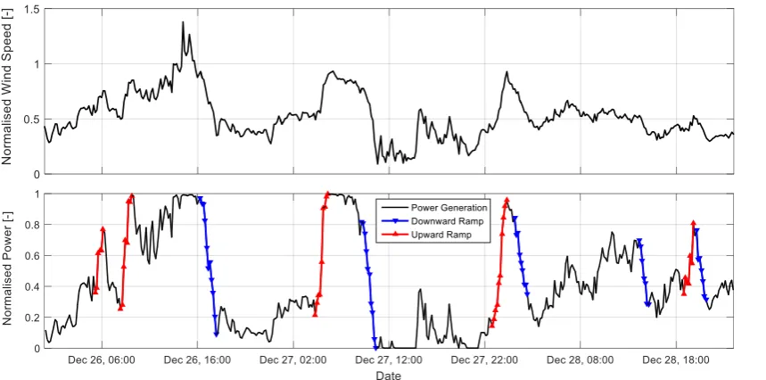
One of the main challenges for the integration of large amounts of wind power into the grid is the occurrence of rapid and strong changes in wind power generation (ramp events). These unexpected events are mainly caused by extreme changes in wind speed and/or direction in a very short period of time, and are frequently associated with the passage of weather fronts. However, the most critical ramp event can occur even for small changes in wind speed. When the wind speed reaches the wind turbine’s cut-out speed, wind turbines shut down automatically for safety reasons, resulting in a large loss of generated power. Despite being critical for the management of the grid, the dynamic allocation of reserves and the stability of the system [9,10] there is no standard definition of a ramp event. It is an individual process of the end-user to define critical ramps and thereby ramp events. A recent publication on the history of wind power ramp forecasting [11] gives an overview of the definitions used in ramp event detection, the meteorological conditions associated to those events and the current forecasting techniques. For most wind power forecasting applications however, the definition of what is critical for an end-user is very individual and dependent on the application as well as the available reserves. For example, a system operator on an island grid or badly interconnected grid needs to have all reserves available within the control zone in order to prevent a critical ramp from causing security issues. A trader may also be very interested in ramp forecasts, as just one event with a large error may cause 95% of the imbalance costs in a month.

Figure 2.Example time series of wind speed and generated power of a single wind turbine with wind ramps marked for a time window of 60 min and a change of power of 40%. Each data point in the time series corresponds to a 10-minute average. Reproduced without modifications from Würth et al. [12].

3. An Overview of Different Applications for Minute-Scale Forecasting in the Wind Industry

The forecast horizon and the parameters that are needed to be forecasted depend on the application of the forecast. Three applications have been identified where minute-scale forecasts of wind speed or power are needed.

1. Wind farm control: Wind turbine and wind plant controllers need the information to optimize, e.g., the power output of the turbines.

2. Physical balancing: They are required by the Transmission System Operator (TSO) in order to optimally operate reserves for the continuous balance of the power system and grid constraint management.

3. Economic balancing: Trading and balancing of wind power in the intra-day or rolling power markets require minute-scale updates of the forecasts with real power output in order to reduce imbalance costs and increase incomes.

It is expected that a next step in the evolution will be storage system planning and optimization in the real-time markets, where the bulk of the energy production will come from renewable energy sources. However, this paper focuses on the applications listed above. In the following each application is discussed in more detail.

3.1. Wind Turbine and Wind Farm Control

Preview information of the wind field is helpful for the control of wind turbines and wind plants. Wind turbine and wind farm controllers need to continuously adjust the operation of the controlled system due to the stochastic changes in the wind inflow. However, traditional controllers are mostly based on feedback and are only able to react to wind changes after the changes already have impacted the turbine dynamics and farm operation. lidar-assisted control algorithms can use the preview information of the wind to proactive adjust and thus improve the wind turbine and wind farm operation by increasing the energy production and reducing structural loads.

1. around 1 s: Feed forward control is used to compensate wind changes to reduce structural loads. For example, the blade pitch, the rotor-effective wind speed is needed only a short time before the wind reaches the rotor to overcome the pitch actuator dynamics [13,14].

2. around 10 s: For Model Predictive Control, the control inputs are optimized to get a chosen compromise of load reduction, energy production, and actuator wear [15,16]. Here, a short time horizon of wind characteristics such as wind speed, direction, and shears is used, typical 5–10 s. 3. around 1–10 min: For yaw control, a wind direction estimation is used to align the wind turbine with the mean wind direction. Yaw control is generally done in the minute scale. In this time scale [17], the yaw signal of lidar systems provides good agreement [18,19].

Active wind farm control is a promising technology to increase the energy production of wind farms [20]. However, flow models are still an important research topic, and the validation of flow models and control strategies are still ongoing. Wind previews for flow control is mainly used in induction control and wake steering for higher energy capture and management of fatigue loading.

Regarding the required preview time for lidar-assisted wind farm control, following classification is useful:

1. around 10 s to 10 min for induction control: Usually the blade pitch angle is used to reduce the power and thus the thrust to weaken wake effects on downstream turbines, which increase the overall production. At partial load this is done by adjusting the “fine pitch” settings which is usually based on a filtered wind speed estimate. Wind previews might help to better adjust the power balancing [21].

2. around 1–10 min for wake steering: The yaw misalignment is used to deflect wakes away from downstream turbines and thus similar preview times compared to the conventional yaw control is useful [22]. A preview of the wind direction might help to better adjust the yaw misalignment in a wind farm.

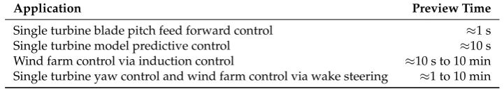
Table1summarizes the preview times for the different applications.

Table 1.Helpful wind preview times for various wind turbine and wind farm applications.

Application Preview Time

Single turbine blade pitch feed forward control ≈1 s

Single turbine model predictive control ≈10 s

Wind farm control via induction control ≈10 s to 10 min Single turbine yaw control and wind farm control via wake steering ≈1 to 10 min

3.2. Power Grid Balancing, Frequency Control and Power Quality in Reserve Market

The focus in this section is on grid balancing, frequency control and power quality embedded in reserve market while the energy market and ancillary services are discussed in the following Section3.3. The balancing term can be employed in a much broader sense in the context of balancing longer time scales. However, in these time scales of mainly energy and reserve market, where balancing actions are scheduled before real time, there are several other means of observations with lower resolutions available [23–25]. However, these are not within the time scales of minute-scale forecasting which is the focus of this section. It should be noted that there are differences in terminology between countries for the same and slightly different balancing actions. In this section, the EU terminology is adopted.

To guarantee the stability of the grid, supply and demand always have to be balanced in spite of the fluctuating power sources. Power quality is achieved if the grid frequency stays within a certain range of a rated value. An imbalance between supply and demand impacts voltage stability and grid frequency, hence there is a need for power balancing [23,26–28].

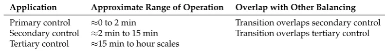
embedded in the reserve market, which are known as primary, secondary, and tertiary controls. The autonomous response of the system to supply/demand imbalances is automatically addressed with primary controls, which is in the scale of microseconds to a few minutes mainly in the scale of seconds. In secondary controls, there are automatic actions and manual actions in scales of seconds to several minutes mainly in the scale of minutes. In tertiary control, both manual and automatic controls are in action from minutes to quarter of an hour to half an hour scales. These are summarized in Table2. All of these actions of balancing are carried out in order to ensure power system quality.

From a market perspective primary, secondary and tertiary reserves are handled differently. Primary reserve is contracted on bi-lateral contracts due to the high-availability requirements. Secondary and tertiary reserves are in some countries traded by auction. The periods range from daily to several days or weeks. Common for or all three reserve products is that the reimbursement is split up into a price for the availability of a specific generation capability and a price for the actual utilization [29].

Wind power and other renewable energy sources create low levels of rotational inertia since these energy conversion systems do not normally act on rotational inertia which has impacts on the power grid frequency. Moreover modern variable-speed turbines are disconnected by inverters from the rotating mass of inertia. Suppliers have started to make changes to create synthetic inertia that can emulate inertia synthetically [30]. Synthetic inertia is about acting to AC frequency, possibly after the loss of a big power plant which makes the grid under-supplied and will result with the AC frequency beginning to fall. This makes accurate short-term forecasting even more important since all of these emulations are dependent on accurate estimation of wind speeds. Hence automatic control for primary and/or secondary controls will certainly benefit from more accurate forecasting on the short-time scales of minutes in control applications.

On another note for the data that is available in the context of this research, any forecast data that is available on scale of microseconds to minutes can be automatically employed in the state estimator of the controller [23,26–28]. The state estimator corrects the state of the system with observational data.

Table 2.Activation of the reserves after an imbalance.

Application Approximate Range of Operation Overlap with Other Balancing

Primary control ≈0 to 2 min Transition overlaps secondary control Secondary control ≈2 min to 15 min Transition overlaps tertiary control Tertiary control ≈15 min to hour scales

3.3. Energy and Ancillary Services Markets

electricity markets and their time lines can be found in [31]. Hence, the importance of the use of updated available minute-scale forecast of wind power has arrived to stay.

Table 3. Lead times and smallest trading blocks for different countries. Sources: Epex [32], Nordpool [33], Energy Exchange Istanbul (EXIST) [34], and BSP South Pool [35].

Country Lead Time Trading Blocks Market

(Minutes) (Minutes)

Austria and Germany 5 15 EPEX Spot

Bulgaria, Denmark, Estonia, Finland, Lithuania,

Norway and Sweden 60 15 NordPool

Belgium, France and the Netherlands 5 60 EPEX Spot

Slovenia 60 15 BSP Southpool

Switzerland 30 15 EPEX Spot

Turkey 90 60 EXIST

In light of this, the forecast process can be split into three components: (1) production of a smooth day-ahead forecast tuned for economic adjustment via the intra-day market, (2) targeting intra-day forecasts for the predictable part of the day-ahead forecast errors and (3) application of forecasts on the minute-scale to manage the wind power generation after gate closure of the intra-day. The two first components correspond to current practices in long-term and short-term processes with some enhancements. The third component is a process running on minute-scale with 1 or 2 h look ahead (e.g., [36]).

Minute-scale forecasts are also necessary when applying to provide ancillary services, secondary or tertiary reserve or balancing capacity for the pool of large utilities. For instance, a recent pilot project in Germany allows wind power generators to participate in the reserve market by down-regulating their production. The possible or available power produced by the wind farms needs to be calculated in one-minute intervals. Furthermore, the standard deviation of the percentage error of the possible or available wind farm power, during the pilot phase, should be less than 5% [37].

4. State-of-the-Art of Wind Power Forecasting

State-of-the-art wind power forecasting methodologies utilize wind speeds from weather forecasts and on-site real-time measurements to compute wind power.

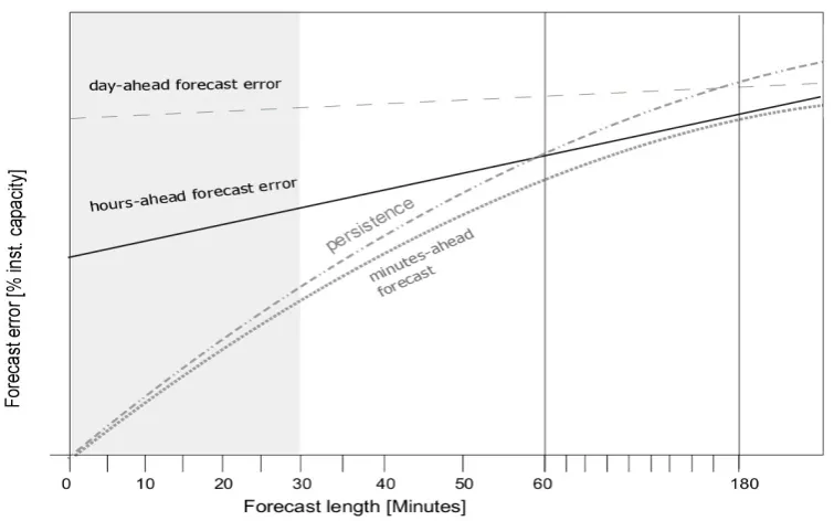
typically around 4–8 h ahead in time. This time span is the typical temporal influence radius of a measurement [38]. The minute-scale and persistence forecasts are both starting at the zero error in their initialization. This is what characterizes this forecasting time scale, where the current state of the power plant is fully known. The steepness of the error growth is also highest for these two forecast techniques due to the decreasing influence of the measurement at the power plant over time. A general industry experience is that a persistence forecast is at the same level as a hour-ahead forecast after around one hour. A minute-ahead forecast should ideally be below the hour-ahead forecast for about 3 h as a thumb rule when evaluating the usefulness of the technique. The time between 1 h and 3 h into the forecast is where the persistence forecast typically reaches the day-ahead forecast error level and loses forecast skill.

Figure 3.Qualitative visualization of the forecast error development over the first hours of a forecast for different temporal forecast techniques.

Figure3illustrated nicely that the margin of possible improvements by minutes-ahead forecasts in the first 30 min of the forecast is rather small in comparison to persistence. Additionally, the average error growth of up to 2% of the installed capacity of a short-term forecast of 15 minute time resolution is rather steep (see Figure3). It is therefore fair to say that the improvement over persistence, which is the objective in the very short time ranges of minutes and hours, is therefore rather modest. This is often used as a reason not to base decisions on forecasts, but rather use persistence, even during ramping, where the persistence forecast is a poor approximation. If the previous 15-min forecast already appears to be off track, then the forecast user cannot be justified in trusting the forecast. Also, the similarity between the average error of a short-term forecast and persistence over the next 15 min strongly indicates whether the short-term forecast performs better or worse than persistence.

A forecast of the steady increase in wind speed from 15 m/s to above the high-speed shutdown point at 25 m/s can also be improved by using wind speed measurements in short-term algorithms. At the high-speed shutdown points (>25 m/s), the wind speed forecast uncertainty is at least 2 m/s even in highly predictable events. The timing of the shutdown is therefore uncertain, even a few minutes before it happens. Wind speed measurements from wind farms reduce this uncertainty significantly. The timing of a high speed shutdown is important for grid security, because there are potentially many Megawatts instantly ramping down. In combination with forecasting on the minute-scale, such wind speed measurements can help to bridge the gap between actual generation and both short-term and long-term forecast.

For wind speeds below the cut-in level there are similar considerations. Mostly, low aggregated wind power generation occurs at low wind speeds. Nevertheless, a large and strong low pressure centre may have near-zero wind speeds from different directions. Both the changes in wind direction and wind speed are better identified by wind speed measurements than wind power measurements. Thus information about wind speeds below cut-in can be crucial for the forecast accuracy near a low pressure system center with highly aggregated wind power generation. During periods of moderate and high generation, wind speed measurements can be used to calculate current potential turbine available generation power or validate the signal of current available power generation sent by the wind generation plant. To conclude, measurements of low, medium and high wind speeds all add value to forecasting, while measurement signals in the steep range of the power curve are least important.

From a technical perspective of the instrumentation, one of the most reported gaps for forecasting hours-ahead and minutes-ahead is the quality of the measurement signals. While wind farm developers have to use calibrated instrumentation and standardized methodologies in order to obtain a bankable level of siting accuracy in the first planning and commissioning phase of a wind project, in the following operational phase the use of meteorological measurements is mostly not defined, documented or standardized. Although the measurements are important in many ways, e.g., situational awareness in extreme events, scheduling and dispatch of generation on power system level, the balancing of large forecast errors, maintenance of instrumentation, there are no standards for the quality of the signals in real-time environments today. For example, if a measurement stops working correctly and sends constant values, a persistence forecast that uses only this data will benefit in performance assessment, while a more advanced minute-ahead forecast that uses other data or models is penalized for providing a more realistic view of the situation. Dependent on the amount of such periods with constant values, this can easily lead to an overestimation of the performance of a persistence forecast in comparison to minutes-ahead forecasts and thereby prevent use and application of minutes-ahead forecasts.

Due to such missing standards and industry guidelines, the main gaps for the use of and collection of meteorological measurements and thereby advances in minute-scale forecasting can be summarized as:

• lack of requirements in the grid codes

• lack of strategy for handling of missing or constant signals from measurements in real-time

• lack of quality of measurements in real-time

5. Review of Methods for Minute-Scale Forecasting

In the previous section we discussed the state-of-the-art in minute-scale forecasting. In this section we investigate instrumentation that can improve forecasting with current techniques and we outline which and how new types of instrumentation and models can be used to improve forecasting on minute scales when persistence can no longer provide a correct picture of the weather conditions.

5.1. Minute-Scale Forecasting Based on Preview Data From Remote Sensing Devices

difficult installation of meteorological masts. With increasing experience and technical advances in technology, remote sensing devices have become viable alternatives. This has also been reflected in the IEC 61400-12-1 2017 standard [39], where such devices have been incorporated as possible instruments to carry out measurements for wind energy applications. A new application for remote sensing devices is forecasting. Especially scanning devices such as scanning lidars and radars which offer the possibility to carry out minute-scale forecasts by delivering high resolution temporal and spacial previews of the upstream wind field of a wind turbine or wind farm. Therefore, the next subsections give an overview of using those devices for forecasting purposes and finally lessons learned with remote sensing instruments in real-time forecasting projects are summarized.

5.1.1. Scanning Lidar-Based Propagation Models

Doppler wind lidars measure the wind speed in direction of the laser beam, also referred to as line of sight (LOS). Depending on the system, the measurement range varies from a few centimeters to several kilometers [40]. Commercial lidars were first used for wind energy applications in the early years of this millennium [41]. Nowadays they have become accepted as an alternative to meteorological masts (met masts) due to cost and ease of installation. Ground based systems are used for site assessment and power performance testing and are now included in international standards [39]. Nacelle-based lidars that can measure upstream of operating turbines, are used for feed-forward control of wind turbines [42]. These systems measure the wind speed several hundred meters upwind, thus forecasting the rotor effective wind speed seconds before it hits the rotor just in time to pitch the rotor blades and reduce loads. A new application for scanning lidars is within wind power forecasting. Commercial lidar manufacturers have increased the range of their systems and compact pulsed scanning wind lidars may now measure the wind speed up to a distance of 10 km over an entire site from one location (see, e.g., [43,44]). There are also systems on the market that measure 30 km and more, but these systems are bigger in size and therefore less suitable for flexible measurement campaigns. The basic idea is to use the spatial and temporal high resolution wind field information measured several kilometers upwind of a wind turbine or wind farm to forecast the power output ahead in time.

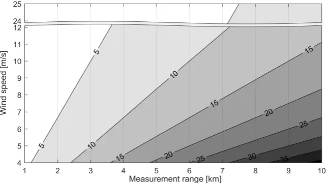
The forecast process (Figure4) is the same for both applications—control and power grid balancing. First the raw lidar data is filtered and the horizontal wind speed and direction is reconstructed from the measured LOS wind speeds. Depending on the number of synchronized lidar measurements, different assumptions need to be made in order to resolve both horizontal wind speed and direction. For instance, a velocity-azimuth display (VAD) retrieval technique is used to resolve both wind speed and direction when only one lidar measurement is available [45]. This method assumes a homogeneous wind field and should only be used in flat terrain where the assumption generally holds true. Then the wind speed in the distance is propagated towards the site by means of a propagation model. The simplest model is based on Taylor’s hypothesis which claims that turbulent structures, so called eddies, are transported with the mean flow without changing their properties. With this assumption the time can be calculated that the wind speed measured in a certain distance needs to reach the turbine or wind farm. Thus the farthest measured distance determines the forecast horizon. The forecasted wind speed at the turbine or farm location is then used either to forecast the power output by means of a power curve model, or as an input to the wind turbine controller.

Power curve

Controller Wind field

reconstruction LOS wind

speeds

Propagation model Wind field

Predicted wind speed/ direction at

turbine

Predicted power

Blade pitch

Figure 4.Forecast process using scanning lidar data.

Figure 5.Forecast- horizon calculated based on Taylor for different wind speeds and measurement ranges; the horizon is given in minutes.

The advantage of scanning lidars is that they offer the possibility to directly measure the wind speed upstream of a turbine. All long-range scanning lidars are pulsed devices, which means that the wind speed information is gathered simultaneously at different measurement distances. Thus the wind flow can be tracked over the span of the measurement and local changes in the wind speed are captured. Modern lidars have compact dimensions of around one cubic meter which allows for flexible measurement campaigns and the installation for instance on the nacelle of a wind turbine or other elevated points such as an offshore substation. Then the scanning of the area on, e.g., a horizontal arc leads to the desired horizontal wind speed information after reconstruction without having to take into account shear effects. When installing the lidar on the nacelle of a wind turbine behind the rotor, it should be noted that due to the blade passage the available data will be reduced, and nacelle vibrations and the tilt angle from the rotor thrust might introduce disturbances in the measurement range and height.

Recent investigations have shown that lidar-based forecasting models were able to predict near-coastal winds better than the benchmarks persistence and ARIMA for a forecasting horizon of 5 min [46]. Another relevant study is Simon et al. (2018) [47] which explores space-time correlations of upwind lidar observations measured on a flat horizontal plane. The study also shows results of a 1–60 min ahead forecast method utilizing the lidar inflow scans which significantly outperforms the persistence method.

sending out laser pulsed that are back-scattered from particles suspended in the air. The wavelength of the back-scattered light shifts relative to the speed of the aerosols according to the Doppler principle [48]. Therefore the device records a noisy signal if not enough or too many aerosols are in the air. It also means that the measurement range fluctuates due to environmental conditions such as fog or rain showers [49]. And as the measurement range determines the forecast horizon, minute-scale forecasts are not possible if the lidar is blind. As a consequence, a fallback solution should be implemented in case the lidar does not provide measurements. Data from other sensors such as radar or drone measurements could be one solution. Using statistical models (cf. Section5.2) or the coupling of the measurements with NWP models (cf. Section5.3) could be another solution. More investigations have to be carried out to determine the optimum conditions for good range measurements of lidars.

Another drawback of lidars so far have been the high costs and the inaccuracies of wind field reconstruction in complex terrain. According to the white paper of the Deutsche Windguard [50,51], especially “in complex terrain sites, influence of the relatively large scanning volume of today’s lidar and SODAR must be carefully considered in terms of its influence on the measurement accuracy...”. This has been a general observation and an ongoing research topic (see, e.g., [41,43,52–55]). In one recent large scale measurement campaign, the Land-Atmosphere Feedback Experiment (LAFE), measurements were setup with multiple synchronized scanning lidars that enable the direct measurements of wind field components (see, e.g., [44,56]). Their instrument setup configuration addressed “the required combination of measurements for advanced studies of the land-atmosphere feedback” with a combination of instrumentation of scanning lidars and surface and airborne in situ measurements that provided the necessary overlap of measured data signals to fill gaps in the instrument’s measurement ranges. This strategy could directly be transferred to the minute-scale forecasting problem in real-time environments and in complex terrain and is also widely applied in the data assimilation of NWP models (see Section5.3).

Another significant obstacle for the application of lidars in the wind power industry is the lack of standard or recommended practices for the use of scanning lidars for wind speed forecasting. More research is needed to find out what the ideal measurement setup looks like, in particular how many lidars are needed and where to place those devices within a wind farm or within a control zone of a system operator. Also, optimal measurement strategies need to be established and transferred to different problem areas and sizes. To that end, different use cases have to be investigated to find out what the best campaign setup and measurement strategy is. Such use cases should include on- and off-shore wind farms of different scales. Recommended practices then need to be consolidated so that the widespread use of lidar for forecasting becomes possible on a commercial level.

5.1.2. Radar-Based Density Models

Radars are remote sensing systems which can determine the position, angle or motion of objects and are being used in multiple applications including traffic control, ocean surveillance, weather monitoring, flight control systems and antimissile systems. Similarly to wind lidars, Doppler radars can be used for wind power forecasting as they are able to determine the velocity of the objects. The working principle is the same as for lidars, but rather than sending light waves, they emit radio waves. Thus, in an environment where meteorological particles with high humidity such as water droplets or ice crystals are present, radars are able to measure the wind speed by determining the motion of the hit particles.

The maximum range that radars can measure is given by the wavelength of the signal emitted, but in this paper we only focus on radars which work on wavelengths that are of interest for minute-scale forecasting of wind power. Thus, we limit our review to radars working between the C-Band and the Ka-band radars, or with a wavelength of 3.2 cm to 8.6 mm.

of the measured wind fields. As with lidars, Doppler radars measure the LOS wind speed. Thus, measuring with one Doppler radar over a defined Plan Position Indicator (PPI) trajectory, the horizontal wind speed can be determined by applying a VAD retrieval technique in the same manner as lidar. To derive the two horizontal wind speed components, two synchronized Doppler radars are needed [57]. The number of publications on the use of Doppler radars for wind energy applications has grown in the last years. Hirth et al. coupled wind farm operational data with wind fields measured by two synchronized Doppler radars (dual-Doppler radar) to further investigate wind farm wake effects [58]. Dual-Doppler measurements of the wake behind an offshore wind farm were also reported by Nygaard et al. [59]. The performance of wind turbines was also validated with dual-Doppler measurements in [60].

First evidence of the promising application of Doppler radar systems for forecasting purposes was documented by Hirth et al. [61]. An extreme wind ramp event observed by the Texas Tech University Ka-band radars at a wind farm in Oklahoma was presented. The authors merged dual-Doppler wind fields with operational data from 32 wind turbines to document the observed transient wind event and its effect on the wind turbines’ performance. They also coupled data from a meteorological tower to analyze the weather conditions that originated the transient event.

Recently, it was shown that Doppler radar observations can be employed to derive minute-scale density forecasts of wind power. In [62] the authors proposed a methodology that uses dual-Doppler radar observations of wind speed and direction in front of a wind turbine to forecast the power generated in a probabilistic framework. In a case study, they predicted the power generated by seven turbines “free-wake” wind turbines in an offshore wind farm. Predictions were generated with a temporal resolution of one minute and with a lead time of five minutes. With their study, the authors showed that the radar-based forecasting model is able to outperform the persistence and climatology benchmarks in terms of overall forecasting skill and generate reliable density forecasts in the case of optimized trajectories.

Figure 6.One of the two Doppler radar units deployed for the BEACon project [59,62].

As with lidars, the same wind power forecasting process can be implemented to derive a wind power forecast. Besides, the fact that they can perform volumetric measurements (wind field measurements at multiple heights), allows to infer further information such as horizontal and vertical wind shear.

However, as with lidars, one of the main obstacles to the adoption of radar as a forecasting tool is the availability of the measurements. The radar measurement principle lies in the backscattering of particles in the air containing high humidity such as water droplets or ice crystals. Therefore, the quality of the measurements relies on the concentration of these particles in the air [57]. Besides, the relatively large dimensions of Doppler radars complicate their installation and reduces the range of possibilities for placing them, especially in offshore environments. The advantage of Doppler radar with respect to lidars is the maximum range that they can measure. However, compared to lidars, the wider beam width of radar results in larger beam spread at large ranges.

5.1.3. Weather Radars for Prediction of Strong Wind Power Fluctuations

Although we have mainly focused on the use of Doppler radars for forecasting applications, weather radars have been also identified as promising candidates for very short-term power forecasting of offshore wind power. Modern weather radars working in the C and X-band measure the intensity of precipitation. They are consequently able to anticipate precipitation fields associated with severe wind speed and power fluctuations with lead times of minutes to few hours, as they can measure up to few hundreds of kilometers, depending on the radar type. The capabilities of anticipating strong wind power fluctuations in offshore wind farms using local weather radars was introduced in [63,64]. In their work the authors were able to track the arrival of precipitation events to the surroundings of an offshore wind farm. These events were highly correlated with the strong observed power fluctuations. The authors also identified shortcomings of the use of weather radars for wind power forecasting, which included: interception of radar waves (cluttering), beam attenuation due to intense precipitation, anomalous propagation of the radar waves during specific atmospheric conditions, underestimation of precipitation reflectivity (beam filling) during convective events, and overshooting at long ranges due to the curvature of the Earth.

5.1.4. Lessons Learned With Remote Sensing Instruments in Minute-Scale Forecasting Projects

Several research projects have been conducted with the goal of integrating remote sensing measurement into real-time forecasting projects. For this purpose not only were scanning devices deployed, but also ground-based profiling devices. In the largest and longest measurement campaigns targeted towards real-time forecasting of wind energy in recent years were two projects funded by the United States Department of Energy. In the Wind Forecasting Improvement Project (WFIP I and II) [65] there were 12 wind profiling radars, 13 sodars and three lidars amongst other meteorological sensors used. Lidars as well as sodars are basic equipment used in meteorological data assimilation today and have been quality checked following meteorological standards through the Meteorological Assimilation Data Ingest System (MADIS) [66]. This was a necessary step in order to integrate the simulations into real-time model forecast systems [67]. In the second project, “Distributed Resource Energy Analysis and Management System (DREAMS) Development for Real-time Grid”, a number of sodars and lidars were used to enhance the Hawaiian system operator’s EMS (Energy Management System) tools for situational awareness of critical events [68]. Here, the instruments were used for the first time as part of an operational management system at a system operator in real-time.

From the above described studies and experimental measuring campaigns as well as real-time testing it can be concluded that remote sensing instruments need to be serviced and maintained similarly to any other real-time instrument. Skilled personnel are required in order for the the devices to run continuously and reliably.

• Lightning protection and recovery strategy after lightning should be ensured.

• Instruments must be serviced and maintained by skilled staff.

• Version control must be maintained for signal processing.

• Measurements must be the originally measured values or technical requirements must include maintenance and software updates.

• Wind data should be measured at a height appropriate for the wind farm, either at hub height or preferable at both hub height and the lowest possible measuring height (e.g., 30 m).

• Remote sensing devices in complex terrain require special consideration.

From studied projects and measurement campaigns, it can be concluded that in active weather conditions, i.e., at the flat range of the power curve as well as under strong precipitation events, it must be expected that met-mast anemometers are more reliable than sodar or lidar devices. From a forecasting and operational monitoring perspective, conditions outside of the instrument’s operating conditions are some of the most critical conditions for grid operation, such as storms with precipitation or high winds. Sodars are more prone to data delivery failures than lidar. In general, however, both devices suffer under non accessibility of measurement information in—for the grid operator—critical situations.

5.2. Statistical Time Series Models

Statistical approaches to forecasting problems mainly rely on deducing patterns from past observational data and extrapolating these relationships to predict future values over a desired time step. With wind energy applications in mind, in this section we consider the task of forecasting a one dimensional time series signal such as a wind speed measurement, or a SCADA source such as wind turbine or wind farm active power signal. The chosen forecast horizon should relate to the time resolution of available input data, and at minimum be one sample (time step) ahead to avoid errors introduced by interpolation. Statistical forecasting methods used on the minute scale are largely identical to techniques employed for longer horizons. The main differences being the temporal resolution of the data and the variability of the physical process being predicted (see Section2).

Data acquisition systems are ordinarily capable of sampling and saving data at high frequency, although historically this data has not always been used nor recorded. For the purposes of minute-scale forecasting, 10-minute or hourly averaged data sets are not sufficient for capturing signal characteristics needed to construct and validate a well performing statistical model. For this reason we recommend that all data generators ensure that they have access to and are logging their high frequency data (both turbine and meteorological sources), and that the instruments are properly maintained. The lower bound of the recorded sampling rate should be at minimum twice the highest frequency in the analog signal you wish to capture, in order to avoid aliasing in the discrete signal transformation (Nyquist sampling theorem). In practice, 1 Hz (1 sample per second) is proposed as a compromise between functionality and transmission/storage considerations. This will allow for future model building and testing which can resolve fluctuations on the minute-scale.

Time series data contrasts to cross-sectional data in that it is naturally ordered in time. Samples which are closer together will normally express a higher correlation than those further apart. This temporal link should be explored through inspection of the autocorrelation and partial autocorrelation function of the time series before beginning any attempts to build a model.

There are often a number of characteristic sub-components embedded in the time series which can be obtained through decomposition techniques in order to normalise samples across time. Examples include differencing an integrated series, removing an overall trend (usually by either mean subtraction or model fitting to obtain the residuals), accounting for cyclic fluctuations, and adjusting for seasonal variations.

not change over time. By implementing the techniques described above, it is possible to transform a non-stationary time series into a stationary one which can be used with traditional forecasting methods.

Benchmarking in any forecasting exercise is crucial. Commonly for forecasting at these short timescales the persistence and climatology models are employed; these simple methods assume that the forecast for the target variable is the most recent available measurement or summary statistics of historical measurements, respectively. Statistical methods for wind speed and power forecasting are typically based on time-series models such as autoregressive [69] (AR) and autoregressive moving average (ARMA) [70,71] models as well as other soft computing techniques such as neural networks [72].

Purely AR models are formulated as a weighted combination of past observations (lags) where the coefficients are normally estimated via ordinary least squares regression. The order of the AR model, or maximum lag, is crucial and can be chosen most simply by inspection of the auto-correlation and partial auto-correlation functions of the signal. Cross-validation or an information criterion provide an alternative method for defining the model order. Domain knowledge of the local meteorological conditions can also be used to extend these simple models. For example, in certain regions the wind/power time series may exhibit strong diurnal trends which would necessitate the inclusion of time-of-day into the model.

Beyond time series models, machine learning techniques also are widely employed. These techniques can be more flexible than classic time series models in terms of easily allowing for more explanatory variables and are typically more naturally able to capture non-linear relationships. It should be noted that this comes at the expense of additional model tuning to optimize algorithm specific hyper-parameters and possible overfitting of the data unless careful cross-validation procedures are followed. Examples include artificial neural networks [72], hybrid multi-models with blending [73] together with feature selection [74], and penalized regression [75].

Artificial neural networks, particularly recurrent neural networks (RNN), have been widely applied for sequence prediction including time-series data. Long short-term memory (LSTM) networks are explicitly designed to capture data patterns of arbitrary lags, and assimilate long-term temporal dependencies [76]. This has led to numerous applications in energy forecasting which outperform traditional time-series modeling approaches. Wu et al. [77] demonstrates such a probabilistic 4-h ahead wind power forecast model employing a LSTM network architecture.

Statistical forecasting models can also be made dependent on the current behaviour of the target time-series or on exogenous variable(s). These are termed regime-switching models and can be based on unobserved regimes [78,79] or by observed regimes like atmospheric conditions [80,81]. It follows that these regimes can be derived from lidar/radar measurements [64]. The benefit of regime switching is that the statistical models can react faster to changing conditions, as opposed to having a fixed coefficient models or by tracking slower changes in behaviour via for instance an online update of the coefficient estimates.

Concurrent information from spatially distributed wind farm or met mast measurements also provide a route for improvements in forecast skill [82]. Multivariate forecasts which encode information on the spatio-temporal dependency of neighbouring sites can be tackled via a vector autoregressive models (VAR) at these time horizons. With an increasing number of sites, making sparse estimates of the coefficient matrices becomes more important, as does estimating them via efficient numerical procedures [83–85].

Forecast uncertainty at these horizons can also be accounted for via probabilistic density forecasts, quantiles, or prediction intervals [86]. These may be generated using parametric assumptions of the forecast distribution shape [69,83] or non-parametric techniques [87,88]. Uncertainty forecasts enable the user to manage risk in decision making and leverage more actionable information from their data, if information content is communicated properly [89].

to evaluate the suitability of statistical methods below this time horizon and at what time range forward facing lidar/radar based systems or hybrid statistical and radar/lidar systems are a more suitable choice.

5.3. Statistical Data Assimilation Based on Physical Models

Data assimilation performs an essential role in the forecasts of wind power systems. While the concept is very inclusive, meaning assimilation of any data with any model, in this section, the term is used in more exclusive sense without addressing statistical time series models. Time series models are a special case of data assimilation where usually non-physical models are taken into consideration. This was discussed in the previous section. The concept is inherent from the fact that neither the model nor the observations are perfect. In order to have an accurate state of the system, the numerical model itself is not sufficient and therefore guidance from observations is required. This is even more so for weather forecast systems, where the system itself is very sensitive to initial conditions and boundary conditions. Data assimilation was first employed in engineering; however, today it is more than an engineering tool.

In summary, in the context of this review article, data assimilation is a technique to adopt multiple measurements and observations of different types into a 3-dimensional model space. In meteorology it is used to generate an initial state of the atmosphere from observations, i.e., an input field, together with boundary conditions to any numerical weather prediction (NWP) model.

Also for the renewable energy production, data assimilation and/or state estimation has an important role, for example in the assimilation of data into the control system on wind turbine or even wind farm level. System operators and wind farm operators require advanced knowledge of ramp-up and ramp-down events [90–92]. In a ramp/extreme event forecasting you want to analyze and use outliers in order to assess the risk of a critical ramp/event that is about to occur, while some data assimilation algorithms can dismiss outliers. The increased frequency of assimilation can address this challenge. The frequency of assimilation is important for ramp prediction, while the challenge comes from the model size and assimilation method chosen for the task; however, simplified models with higher frequencies can be adapted for the applications discussed here.

The work on data assimilation spans many disciplines and several decades in which many different methods have been developed to adapt the state of the atmosphere in numerical weather prediction models to large sets of measurements [93,94]. The initial development of data assimilation has started as an objective analysis (e.g., [95,96]), which is also referred to as successive correction methods.

This work was followed by optimum interpolation (OI) (e.g., [93,97]). Optimal Interpolation (OI) methods have lead to development of variational methods in data assimilation, where constraints were introduced in variational data assimilation methods. These methods are namely 1DVAR, 2DVAR, 3DVAR (e.g., [98,99]) and 4DVAR (e.g., [100,101]) where D stands for Dimension. Variational approaches can be also formulated in the context of a Bayesian problem.

employs Monte-Carlo methods to estimate the background covariance errors to introduce nonlinearities to Kalman filter (e.g., [102,107–109]).

Möhrlen et al. [36] found that some of the Kalman filter limitations in a meteorological context are, however, not a limitation in the wind power context, because the area of observational distribution is rather small, even if the area spans over an entire country. In atmospheric data assimilation the measurement data used is spread widely in space (globally), but is mostly sparse in time. In a wind power context, observations are concentrated in small areas with high time resolution. A classical KF approach would not make sense as models would have to generate forecasts in a small area, which is undesired, or it would require unrealistically many computing resources and observational input of meteorological variables [36]. The physical based ensemble prediction methods, especially the multi-scheme approach, has been found as the most efficient method due to its ability to generate spread that has a physical/meteorological meaning in any time step with a much smaller ensemble size [110].

One non-exclusive approach that can address the above approximations on linearities and Gaussianity is particle filter (PF); however, it brings computational cost with it [111]. The computational cost is also related to ensemble size; however, this can be addressed adaptively with careful selection of ensembles introduced by Uzuno ˘glu [112,113]. The computational complexity in the above summarized methods can be addressed in the subspace of ensembles that was one of the focuses of the Maximum Likelihood Ensemble Filter (MLEF) that employs ensembles in the pre-conditioner. The computational time is reduced by optimizing a nonlinear cost function in low dimensional sampling space for Hessian information through maximum likelihood practice which also addresses the stochasticity and the discontinuity. This method has been applied to many disciplines such as power systems as well as to the wind energy industry [27,114]. In the workshop, the successful application of this method to second scales were presented.

5.4. Extreme Event Forecasting Models

Extreme events in a meteorological sense are events that deviate from the mean and exceed beyond specific threshold limits. In the power system, extreme events can occur under meteorological average conditions as well and not be considered extreme, when meteorological threshold values, such as wind speed, are exceeded. The differences are mainly due to constraints in the transmission lines and the supply and demand relationship. Only in areas where wind turbines shut down due to high wind speeds- so called high-speed shutdowns, can such wind speeds challenge both life and the ability to safely control the grid.

The way to deal with extreme events in both meteorology and the power industry is by applying uncertainty forecasts that provide an objective measure of the possible extreme. Deterministic forecasts cannot serve such situations, as they are tuned for best average conditions, i.e., in the setup, statistical training and model output statistics, outliers and extremes are filtered out. While statistical approaches can be used in many life science applications, in power system applications it is crucial to employ an approach that provides a valid uncertainty of the forecast inclusive of extremes in every hour of the forecast. Such extreme forecasts must be established based on probabilities computed from a probabilistic prediction system that can take the spatial and temporal scales into consideration in order to capture the temporal evolution and spatial scale of, e.g., low pressure systems that contain wind speeds leading to large scale shut-down of wind farms.

suitable solutions for a decision process. They can be computed for very critical and less critical events, depending on the end-users’ requirements.

In meteorology the use of sophisticated observational instrumentation for data assimilation problems is an ongoing transformation throughout the last decades. As new technologies become available that in some way are able to reflect some part of the atmospheric system, where the model systems require parameterizations, such instrumentation is usually tested in research campaigns and then deployed at specific locations (e.g., [110,115–118]). Transferring this knowledge to the assimilation of wind power observations that are irreversible in their nature is more complex. Nevertheless, a unified methodology that is able to decide on the value of an observational signal and it’s impact on the total system is required to solve this task.

In Section5.1.2we learned that radar measurements can be used for forecasting, but require transformation algorithms to be useful for the forward propagation of the data signals. The Kalman Filter techniques are practical approaches that have inherent capabilities to transform such data signals and use them in convective-scale data assimilation tasks (see, e.g., [117,118]).

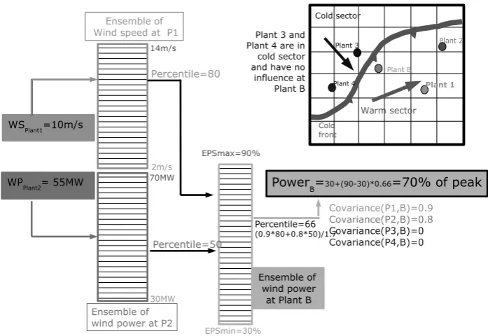
Figure 7. Functionality of the inverted Ensemble Kalman Filter when using different kind of measurements. P stands for Plant.

5.5. Overview of Methods for Minute-Scale Forecasting

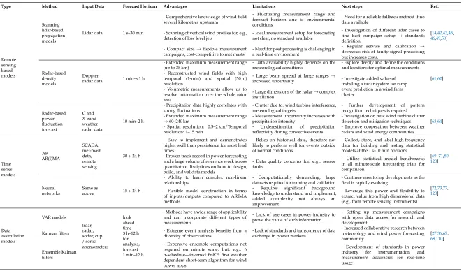
Table4provides an overview and summary of the different minute-scale prediction methods, their forecasting horizons as well as advantages and limitations to the adoption of the methods. It also lists next steps that are suggested as a way to overcome the limitations.

During the discussions at the workshop and also whilst writing this paper, it became clear that as of now we are not in a position to recommend a minute-scale forecasts method that performs well in all conditions and for all use cases. Depending on the data input and the method, there are certain advantages and limitations that are inherent to the respective forecast types and methods. Remote sensing-based models for example work with preview data of the wind field several kilometers upstream of a wind turbine, but rely on the data availability of the remote sensing device which strongly depends on atmospheric conditions. Time series models are flexible in terms of input data, have a proven track record in power forecasting and have been used to a great extent across multiple disciplines. However, they rely on historical data and are therefore not likely to perform well for events outside of normal conditions. Data assimilation models have a wide range of applicability and can incorporate different types of measurements, but there is a lack of experience in the wind power industry.

Table 4.Overview of methods for minute-scale forecasting.

Type Method Input Data Forecast Horizon Advantages Limitations Next steps Ref.

Remote sensing based models Scanning lidar-based propagation models

Lidar data 1 s–30 min

- Comprehensive knowledge of wind field several kilometres upstream

- Fluctuating measurement range and forecast horizon due to environmental conditions

- Need for a reliable fallback method if no data available

[14,42,43,45,

46,49,50] - Scanning of vertical wind profiles for, e.g.,

detection of low level jets

- Ideal measurement setup for forecasting not clear, no standard available

- Investigation of different lidar cases to find best campaign setup→ standards definition.

- Compact size→flexible measurement campaigns, cost-competitive to met masts

- Need for post processing is challenging in a real-time environment

- Regular service and calibration → decreases risk of faulty signal processing but increases costs.

Radar-based density models

Doppler

radar data 1 min–<1 h

- Extended maximum measurement range (up to 35 km)

- Data availability highly depends on the meteorological conditions

- Explore deeply and define the conditions and locations for optimal measurements

[61,62] - Reconstructed wind fields with high

temporal (1-min) and spatial (50 m) resolution

- Large beam spread at large ranges→

increased uncertainty - Investigate added value of_{installing a radar system for ramp}

event prediction in a wind farm cluster

- Volumetric measurements allow us to resolve information over the whole rotor area

- Large dimensions of the radar→complex installation Radar-based power fluctuation forecast C and X-band weather radar data

10 min–2 h

- Precipitation data highly correlates with strong fluctuations

- Clutter due to: wind turbine interference, meteorological targets

- Further development of pattern recognition techniques is required

[63,64] - Extended maximum measurement range

→60–240 km

- Measurement uncertainty increases with precipitation intensity

- Investigation on new wind turbine clutter detection and mitigation techniques - Spatial resolution: 0.5–2 km/Temporal

resolution: 1–15 min

- Underestimation of precipitation reflectivity during convective events

- Improve cooperation between weather radars and wind energy communities

Time series models AR AR(I)MA SCADA, met-mast data, remote sensing

30 s–24 h

- Easy to implement and demonstrates higher skill than persistence for most lead times

- Relies on historical data, therefore not likely to perform well for events outside of normal conditions

- Collect, store, and label high-frequency data for building and testing statistical models at the 1 s–10 min horizons

[69–71,80,

120] - Proven track record in power forecasting

and a large volume of reference work across quantitative disciplines on how to design, build, and validate models

- Data quality concerns for, e.g., sensor faults

- Utilize statistical model benchmarks in all minute-scale forecasting trials for comparison

Neural networks

Same as

above 15 s–24 h

- Ability to learn complex non-linear relationships

- Computationally demanding, large datasets required for training and validation

- Continue monitoring developments as the field is rapidly evolving

[72,73,77,

120] - Flexible model construction in terms

of inputs/outputs compared to ARIMA methods

- Requires significant background knowledge to understand and implement, added complexity not always an improvement

- Leverage this power and flexibility to extract value from high dimensional data (e.g., from remote sensing instruments)

Data assimilation models VAR models lidar, radar, sodar, cup / sonic anemometers look ahead time 3 h–12 h for analysis, forecast 1 min–12 h

- Methods have a wide range of applicability and can incorporate different types of measurements

- Lack of use cases in power industry to prove the value of such information

- Setting up measurement campaigns with open data access for research and development

[27,36,67,

68,110] Kalman filters - Extreme event analysis benefits from a_{diversity of observations} - Lack of standards and transparency of data_{exchange in power markets}

- Increased collaborative research between meteorology and wind power forecasting community

Ensemble Kalman filters

- Expensive ensemble computations not required on minute scale, but, e.g., 6 h-schedule—inverted EnKF: first weather dependent short-term algorithm for wind power apps

6. Challenges for the Implementation of Minute-Scale Forecasting in Large Energy Systems

There are several use cases for predictions shorter than 1 to 2 h. In Australia, the system runs on a 5-min schedule [121] and requires renewable energy and load forecasts on those time scales. In Germany, renewable energy plants can be pre-qualified to participate in the reserve market, and need to predict their possible power with less than 5% error in the pilot phase and less than 3.3% in the implementation phase. This is calculated in one-minute intervals. In Denmark, with hourly wind penetrations of over 140%, the grid is run proactively in hourly steps, predicting the imbalance and reacting accordingly on the basis of spatio-temporal forecasts [122]. So the use cases for minute scale forecasts are present, and the best forecasts require upstream information in real time.

In a large energy system with moderate penetration from wind sources, a system operator can choose to outsource balancing of wind. This is the approach chosen widely in central Europe. A major reason behind the liberalized strategy in Europe is a wish to make the market more competitive which has happened faster than anybody expected in both Denmark (2009) and Germany (2012) [123] with the result of lower spot market prices in the NordPool market and the German-Austrian component of EPEX.

The difference between a TSO and a power trader’s prioritized optimization lies in the target horizon. The trader is looking up to several weeks ahead, while the TSO’s optimization horizon is over the entire year. In particular once the power trading is privatized and handled by private balance responsible parties, then the TSO lacks information about the generation and must rely on the information from the trading companies. In Germany, the TSOs have today little control of renewable energy generation and rely on out-sourced solutions for critical system information to a large degree which has not been considered acceptable for many years from a system security perspective.

Although Germany has the highest capacity of wind and solar generation in Europe, it is apparent that the system lacks information for optimization. This is seen in frequent downregulation of wind farms during day-time and recovery during the middle of the night, often many hours after the wind has dropped again. This process has become highly inefficient in recent years, because there are no requirements for wind farms to provide real-time data to the system operator.

The German experience shows that wind energy loses efficiency and value unless there are obligations for wind farms to provide data required by various forecasting and system operation processes.

Based on this experience, it is crucial to define standards regarding the setup and maintenance of instrumentation, collection and provision of data, as well as required quality of data. Beside the standards, in transparent markets the grid codes should also contain a clear definition about the rights on the use and the obligation to provide the data. Without such regulations, the required quality is hard to achieve in order to improve forecasts. Corrupt and wrongly calibrated instrumentation can do more damage to a forecast than not having data. This is one of the greatest challenges at present and the reason for slow progress on minute-scale forecasting. Especially in large systems such as Germany with many thousands of individual wind turbines and small wind farms, this is a difficult challenge to overcome. Nevertheless, the need to make appropriate changes to the grid codes is the same for all markets.

7. Conclusions

Three applications were identified that can benefit from minute-scale forecasting and their respective forecasting horizons. Wind turbine and wind farm controllers need wind speed forecasts with the shortest horizon to optimize the turbine and farm operation. The task of balancing the power grid, and finally optimizing energy markets which rely heavily on precise wind power forecasts on a slightly longer time scale as well.

To carry out forecasts that range from 1 second to 60 min, forecasters have the choice between different methods (Figure8). In our discussions at the workshop and this review paper we differentiate between using preview data from remote sensing devices, time series models that deduce patterns from observational data to predict future values and finally methods that are based on data assimilation into physical models. These assimilated data can originate both from remote sensing devices or other existing observational data sources i.e., meteorological masts and wind turbine data.

Forecast horizon

1s 1min 10min 30min 1hour

Wind turbine and wind plant control Power grid balancing Scanning lidar-based models

Statistical methods

NWP models + measurements

Methods

Applications

5min

Energy and ancillary services market Radar-based models

Figure 8.Overview of forecast horizons of different wind energy applications and forecast methods in the second and minute scale.

By investigating more deeply the respective methods it became clear that they all have advantages, but also limitations that need to be overcome in order to achieve reliable forecasts for commercial use. The following list provides an overview of focus areas for the near future to advance further with minute-scale forecasting: