A kernel method for non-linear systems identification – infinite degree volterra series estimation

This is a repository copy of A kernel method for non-linear systems identification – infinite

degree volterra series estimation.

White Rose Research Online URL for this paper:

http://eprints.whiterose.ac.uk/74496/

Monograph:

Wan, Y., Dodd, T.J. and Harrison, R.F. (2003) A kernel method for non-linear systems

identification – infinite degree volterra series estimation. Research Report. ACSE

Research Report no. 842 . Automatic Control and Systems Engineering, University of

Sheffield

[email protected] https://eprints.whiterose.ac.uk/

Reuse

Unless indicated otherwise, fulltext items are protected by copyright with all rights reserved. The copyright exception in section 29 of the Copyright, Designs and Patents Act 1988 allows the making of a single copy solely for the purpose of non-commercial research or private study within the limits of fair dealing. The publisher or other rights-holder may allow further reproduction and re-use of this version - refer to the White Rose Research Online record for this item. Where records identify the publisher as the copyright holder, users can verify any specific terms of use on the publisher’s website.

Takedown

If you consider content in White Rose Research Online to be in breach of UK law, please notify us by

A KERNEL METHOD FOR NON-LINEAR SYSTEMS

IDENTIFICATION – INFINITE DEGREE VOLTERRA SERIES

ESTIMATION

Yufeng Wan, Tony J. Dodd, and Robert F. Harrison

Department of Automatic Control & Systems Engineering

The University of Sheffield, Mappin Street, Sheffield S1 3JD, UK

{

y.wan, t.j.dodd, r.f.harrison

}

@sheffield.ac.uk

Research Report No. 842

Abstract

Volterra series expansions are widely used in ana-lyzing and solving the problems of non-linear dynami-cal systems. However, the problem that the number of terms to be determined increases exponentially with the order of the expansion restricts its practical application. In practice, Volterra series expansions are truncated severely so that they may not give accurate represen-tations of the original system. To address this problem, kernel methods are shown to be deserving of exploration.

In this report, we make use of an existing result from the theory of approximation in reproducing kernel Hilbert space (RKHS) that has not yet been exploited in the systems identification field. An exponential kernel method, based on an RKHS called a generalized Fock space, is introduced, to model non-linear dynamical sys-tems and to specify the corresponding Volterra series expansion. In this way a non-linear dynamical sys-tem can be modelled using a finite memory length, infi-nite degreeVolterra series expansion, thus reducing the source of approximation error solely to truncation in time. We can also, in principle, recover any coefficient in the Volterra series.

1

Introduction

Volterra series models are widely used in analyzing and solving the problems of non-linear dynamical sys-tems. The term Volterra series derives from the work of Vito Volterra, an Italian mathematician, at the end of the nineteenth century, the idea of which can be re-garded as an extension of the linear convolution model. Volterra series have been shown to provide a good rep-resentation for a wide range of non-linear systems [2]. Without the involvement of the previous, predicted out-put signals, such a model can give a relatively accurate prediction of the output over the domain of interest for systems of “fading memory” type [2], assuming we can measure the input signals exactly. Because of this

and some other practical advantages such as their being linear-in-the-parameters [9], much has been done in the development and application of Volterra series models. At the same time, a noticeable shortcoming restricts the practical use of even truncated Volterra series because they involve exponentially many parameters. Thus, in practice, only “small” models have been found to be useful with a concomitant loss of precision. The use of kernel methods for finite degree, finite length Volterra series estimation has already been addressed [8, 5, 3, 4]. This report is primarily concerned with discrete-time, finite length, infinite degree Volterra series ex-pansions. A method based on exponential kernels is used to model non-linear dynamical systems and to de-termine the parameters of the corresponding Volterra series. The next section gives the theoretical basis of the subsequent discussion. The particular Generalized Fock (GF) space, F, and the corresponding kernel, k, are constructed. Proof that k is a reproducing kernel andF is its reproducing kernel Hilbert space (RKHS) is given. In section 3 the method of computing infinite degree Volterra series expansions using the kernel con-structed in section 2, is discussed. The problem of how to recover the original Volterra series from the kernel is discussed in section 4, and, in section 5, two synthetic system identification examples are given. Finally, we discuss the limitations and potential of the method.

2

Generalized Fock Spaces

Consider a discrete-time, finite length1_{, infinite}

de-gree Volterra series expansion

y(u) =h0+

∞ X

n=1

( _M X

m₁=1 · · ·

M

X

mn=1

hn(m1, . . . , mn) n

Y

j=1

umj

)

,

(1)

1

where

u= [u1, . . . , uM] T

and M is the memory length. A sufficient but not necessary condition that guarantees the convergence of Eq.(1) is that [9]:

M

X

m₁=1

M

X

m₂=1

· · ·

M

X

mn=1

|hn(m1, m2, . . . , mn)|<∞ (2)

A GF space,F, can be constructed [6], consisting of the elements,f,

F: f =hf0+

∞

X

n=1

1

n!fn, (3)

in which thefn, given by

fn(u) = M

X

m₁=1

· · ·

M

X

mn=1

hfn(m1, . . . mn) n

Y

j=1

umj (4)

completely characterizef.

We then define the inner product [7] in the specified GF space,F, as:

< f, g >F= ∞

X

n=0

pn

n! (fn, gn)n, (5)

where

(fn, gn)n = h f 0h g 0 (6) + M X

m₁=1

M

X

mn=1

hfn(m1, . . . , mn)hgn(m1, . . . , mn).

In Eq.(5),P =©

p0 , p1

, . . . , pn_{, . . . , p}∞ª

denotes a set of weighting constants, in whichpis a constant chosen according to prior knowledge and satisfying the con-vergence condition given by Eq.(2). The relationship betweenpandhn will be established later.

We then construct an exponential kernel

k(u, v) = exp µ

< u, v >l2

p

¶

(7)

in which< u, v >l₂ denotes a dot product inl2,

< u, v >l₂=uTv= M

X

i=1

uivi. (8)

According to the theory of Taylor Series, we know

that ex =

∞

X

n=0

xn

n!. So the exponential kernelk can be rewritten as

k(u, v) =

∞

X

n=0

1

n!

(< u, v >l2)

n

pn = ∞

X

n=0

1

pn_n!(< u, v >l2) n

(9) We can now prove thatkis a reproducing kernel in

F through the following two steps:

1. For a fixed input sequence,u, we substitute Eq.(8) into Eq.(9) such that

k(u, v)

= ∞ X n=0 1 n! ³ PM

i=1uivi

´n

pn

= 1 +

∞ X n=1 1 n!   1 pn M X

m₁=1

· · ·

M

X

mn=1





n

Y

j=1

umj

n

Y

j=1

vmj 

 



= 1 +

∞ X n=1 1 n! ( M X

m₁=1

· · ·

M

X

mn=1

    1 pn n Y j=1

umj 



n

Y

j=1

vmj      (10)

wherehkn is defined as follows:

hkn=

½

1 , n= 0;

1

pn

Qn

j=1umj , n= 1,2, . . . ,∞.

(11)

Substituting Eq.(11) into Eq.(10), we get

k(u, v) =

∞

X

n=0

1

n!kn(v) (12)

in which

kn(v) =hk0+

M

X

m₁=1

· · ·

M

X

mn=1

hkn(m1. . . mn) n

Y

j=1

vmj.

(13) Eqs.(12), (13) are of the general forms, (3), (4), which meansk(u, .)∈ F.

2. For every f ∈ F, we have

< k(u, .), f(.)>F= ∞

X

n=0

pn

n! (kn, fn)n. (14)

If we replace (kn, fn)n in Eq.(14) with Eq.(7),

hk(u, .), f(.)iF can be re-written as follows:

< k(u, .), f(.)>F

= ∞ X n=0 pn n! Ã

hk0h

f

0+

M

X

m1=1

· · ·

M

X

mn=1

hknh f n

!

= hk0h

f 0+ ∞ X n=1 pn n!   M X

m1=1

· · ·

M

X

mn=1

1

pn n

Y

j=1

umjh

f n





= hf0+

∞ X n=1 1 n!   M X

m₁=1

· · ·

M

X

mn=1

hfn n

Y

j=1

umj 

 (15)

in which we have usedhk

0 = 1. Recalling the

< k(u, .), f(.)>F = ∞

X

n=0

1

n!fn(u)

= f(u) (16)

Eq.(16) demonstrates the reproducing property of the kernel,k(u, v).

The functionk:RM ×RM →R+ having the above

two properties is called the “reproducing kernel” [1] of the spaceF. Equipped with such ak,F is known as a RKHS. The characteristic of such a kernel,k, is encom-passed in the Moore-Aronszajn theorem:

Theorem 2.1 [10] To every RKHS there corresponds a unique positive-definite function (the reproducing ker-nel) and conversely given a positive-definite function,k, onRM we can construct a unique RKHS of real-valued functions onRM with kas its reproducing kernel.

Property 2 above is very useful and will be utilized in the next section to get an important result.

Given that the kernel, k(u, .), belongs to the GF space, F, functions in F corresponding to the infinite degree Volterra series expansions, Eq.(3), can now be expressed in terms of the kernels,

f(u) = N

X

i=1

aik(ui, u) (17)

whereN is the number of samples andai ∈R.

3

The Best Approximation of The

Orig-inal Volterra Series Expansion

It is well known that, given (16), the best approxi-mation, ˆy, of the original Volterra series expansion, y, is given by the projection of y in the closed subspace ofF spanned byk(u1, .), . . . , k(uN, .). Therefore, ˆy is given by

ˆ

y(u) = N

X

i=1

aik(ui, u) (18)

where

ui = [ui1, . . . , uiM] T

.

In Eq.(18), a : a = [a1, . . . , aN]T is the coefficient vector that we need to specify. It can be obtained by the following equations [7]:

a=K−1y, (19)

where

y= [y1, . . . , yN] T

andKis the kernel Gram matrix,

Kij =k

¡

ui, uj

¢ = exp

µ_{< u}

i, uj>l2

p

¶

. (20)

Note that it has been proven [11] that, under some restrictions, the kernel Gram matrix,K, is nonsingular, providing a unique solution to (19).

Theorem 3.1 [11] If ui, i = 1,2, . . . , N, are distinct elements ofRM_{, then theN×N matrixK,}

Kij = exp

µ_{< u}

i, uj >l2

p

¶

, (21)

is nonsingular.

The above statements give the idea and the way to com-pute the infinite degree Volterra model with the expo-nential kernel,k, given by Eq.(7). In the following sec-tion, we will discuss how to recover the terms of the original infinite degree Volterra series model, which is valuable for the analysis and interpretation of systems in practice.

3.1

Numerical Considerations

We note that Theorem 3.1 gives a theoretical guar-antee for the existence of a unique solution, ˜a, but, in practice, even in the noise free case, numerical sen-sitivity may present a problem and we often need to solve Eq.(19) via the pseudo-inverse or by introducing Tikhonov (ridge or weight decay) regularization (with parameter,ρ), thus ˜a = (K+ρI)−1y. The reason for this is that the kernel matrix,K, typically becomes ill-conditioned as the number of samples becomes large. It can be seen from Eq.(17) that the predicted out-put,f(u), is the weighted sum of the kernels,k(ui, u). As the sample size,N, increases, depending on the nu-merical precision of the computer used to run the pro-gramme, at least two rows of the kernel Gram matrix,

K, will tend to co-linearity. Since our ultimate pur-pose is system identification in a noisy environment, we adopt regularisation and accept a biased solution.

4

Recovery

of

The

Infinite

Degree

Volterra Model

Volterra series models are widely used in analyz-ing non-linear systems because they contain important characteristics of the physical systems and are qualita-tively well-behaved, like linear finite impulse response models. At the same time, an infinite degree Volterra model can, in principle, give an arbitrarily accurate rep-resentation for the corresponding fading memory, non-linear system, so the recovery of the model is of great importance for us in many cases.

Substituting Eq.(8) and (9) into (18), we have

ˆ

y(u) = N

X

i=1

aik(ui, u) = N

X

i=1

ai

"∞

X

n=0

1

n!pn

à M

X

m=1

uimum

!n#

.

We can expand the polynomial³PM

m=1uimum

´n in Eq.(22) to rewrite it as

ˆ

y(u) = 1

p0

N

X

i=1

ai+ M

X

m₁=1

à 1

p1

N

X

i=1

aiuim₁

!

um₁

+ M

X

m₁=1

M

X

m₂=1

à 1 2!p2

N

X

i=1

aiuim₁uim₂

!

um₁um₂

+· · ·+ M

X

m₁=1

M

X

m₂=1

· · ·

M

X

mn=1

à 1

n!pn N

X

i=1

aiuim₁. . . uimn !

um₁. . . umn

+. . . (23)

Given that

hn= 1

n!pn N

X

i=1

ai n

Y

j=1

uimj.(n= 0,1, . . . ,∞), (24)

Eq.(23) is equivalent to the following,

ˆ

y(u) =h0+

∞ X

n=1

( _M X

m₁=1 · · ·

M

X

mn=1

hn(m1, . . . , mn) n

Y

j=1

umj

)

,

(25)

which is the same as the form of the infinite degree Volterra series expansion, (1). Therefore, we find that the original infinite degree Volterra series model can be recovered from the kernel model. The coefficient of each term,hn, is given by Eq.(24).

5

Example

We choose examples of two Wiener-type systems (see figure 1) to illustrate the method. The first requires a model of infinite polynomial degree but has a finite memory length and is thus exactly matched to our so-lution. The second has infinite memory length and the same non-linearity. The linear block is designed, for il-lustrative purposes, so that the number of sizeable com-ponents of its impulse response function is small. We only examine the first and second order generalised fre-quency response functions.

5.1

Finite Memory, Infinite Degree Wiener

Model

G(z) f(v)

[image:5.612.49.555.89.528.2]

u(t) v(t) y(t)

Figure 1: Linear-Non-linear Wiener model

The process is given as

yt=

e−v_t2

1 +e−5vt (26)

vt= 0.5ut+ 2.5ut−1+ 1.7ut−2. (27)

i.e. M = 3. The Taylor series ofytin terms ofvt is

yt= 0.5 + 1.25vt−0.5vt2+O

¡

v3

t

¢

. (28)

Substituting Eq.(27) into (28), we have

yt = 0.5 + 1.25 (0.5ut+ 2.5ut−1+ 1.7ut−2) −0.5 (0.5ut+ 2.5ut−1+ 1.7ut−2)

2

+O¡

v3

t

¢

. (29)

The corresponding first and second order Volterra kernels are

h1=

£

0.625 3.125 2.125¤

h2=−





0.125 0.625 0.425 0.625 3.125 2.125 0.425 2.125 1.445 

.

Without introducing noise, the model was simulated to generate (1998 + 2M) pairs2_{of input-output samples}

in which the input signal sequence,{ut}, was uniformly distributed between 0 and 0.1. The regularization pa-rameter, ρ, and the parameter, p, were chosen to be 1×10−9_{and 0}

.009, respectively. This value ofρwas se-lected as the smallest one that avoided ill-conditioning ofK. pwas chosen because it led to the minimum dif-ference between the Volterra kernels of the true and the estimated model. AssumingM was known, we applied the exponential kernel method to estimate the system. The resulting performance of the simulation in the time domain (not shown) has a mean square error on the order of 10−11

.

The estimated first and second order Volterra kernels are

ˆ

h1=

£

0.6246 3.1230 2.1236¤

ˆ

h2=−





0.1272 0.6020 0.4048 0.6020 3.0123 2.0543 0.4048 2.0543 1.3943 

.

Theoretically, the infinite degree, finite length Volterra series discussed in this paper can simulate the target model exactly. The difference between the true values and the estimated values was caused by machine imprecision and bias incurred through regularization. The corresponding first and second order generalised frequency responses are shown as follows.

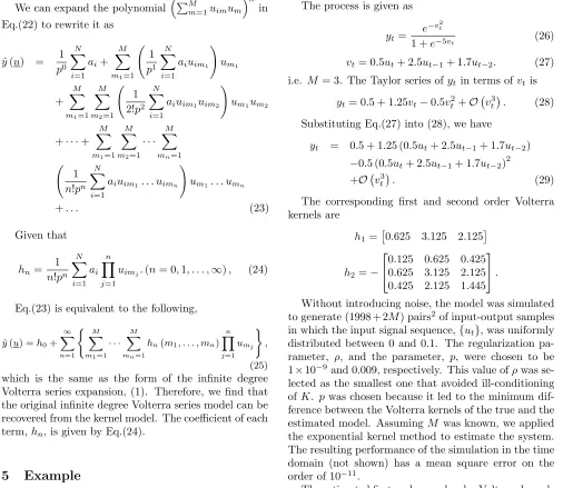
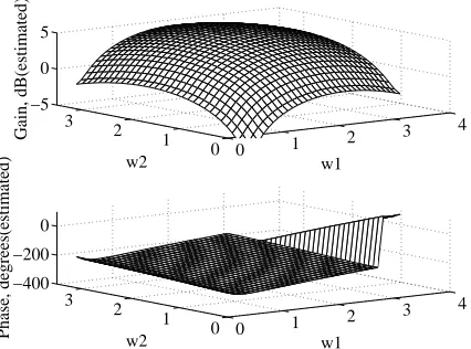
As shown in figure 2, the estimated gain and phase of the first order frequency response are indistinguishable. In the second order frequency response figures 4−6, the maximum absolute errors in the gain and phase are approximately 1.3dB and 11 degrees, respectively.

2

0 1 2 3 4 −5

0 5 10

w

Gain, dB

0 1 2 3 4

−400 −200 0

w

[image:6.612.54.270.89.255.2]

Phase, degrees

Figure 2: Target first order frequency response (‘–’) specified in Eqs.(26), (27) and the estimate (‘- -’) with

M = 3, p= 0.009

0 1 2

3 4 0

1 2 3 −5

0 5

w1 w2

Gain, dB(true)

0 1 2

3 4 0

1 2 3 −400 −200 0

w1 w2

[image:6.612.310.526.101.253.2]

Phase, degrees(true)

Figure 3: Target second order frequency response spec-ified in Eqs.(26), (27)

0 1 2

3 4 0

1 2 3 −5

0 5

w1 w2

Gain, dB(estimated)

0 1 2

3 4 0

1 2 3 −400 −200 0

w1 w2

Phase, degrees(estimated)

Figure 4: Estimated second order frequency response withM = 3, p= 0.009

0 1 2

3 4 0

1 2 3 −5

0 5

w1 w2

Gain, dB(error)

0 1 2

3 4 0

1 2 3 −400 −200 0

w1 w2

[image:6.612.53.266.335.486.2]

Phase, degrees(error)

Figure 5: Differences between the true and the esti-mated gain and phase of the second order frequency response for the finite memory, infinite degree Wiener model

5.2

Infinite

Memory,

Infinite

Degree

Wiener Model

The structure of the model is the same as above. But in this case, the linear process component is given as

vt=−0.5vt−1−0.1vt−2+ 0.5ut−1. (30)

Thus, theoretically, this model has infinite memory length. But as shown in figure 6, the linear impulse response sequence fades in 5 to 7 seconds.

Impulse Response

Time (sec)

Amplitude

0 2 4 6 8 10

−0.3 −0.2 −0.1 0 0.1 0.2 0.3 0.4

Figure 6: The impulse response of the linear block spec-ified by Eq.(30)

By substituting Eq.(30) into (28), the first and sec-ond order Volterra kernels of the model can be com-puted,

h1=

£

0 0.625 −0.3125 0.0938 · · ·

· · · −0.0156 −0.0016 0.0023 −0.0010¤

[image:6.612.309.521.474.643.2] [image:6.612.54.267.546.704.2]

h2=



          

0 0 0 0 · · ·

0 −0.1250 0.0625 −0.0188 · · ·

0 0.0625 −0.0313 0.0094 · · ·

0 −0.0188 0.0094 −0.0028 · · ·

0 0.0031 −0.0016 0.0005 · · ·

0 0.0003 −0.0002 0 · · ·

0 −0.0005 0.0002 −0.0001 · · ·

0 0.0002 −0.0001 0 · · ·

· · · 0 0 0 0

· · · 0.0031 0.0003 −0.0005 0.0002

· · · −0.0016 −0.0002 0.0002 −0.0001

· · · 0.0005 0 −0.0001 0

· · · −0.0001 0 0 0

· · · 0 0 0 0

· · · 0 0 0 0

· · · 0 0 0 0



          

.

The input samples, {ut}, are uniformly distributed between 0 and 1 andM = 5. The parameters,ρandp, are set to be 1×10−5 _{and 1, respectively. Again, the}

parameter configuration was determined in terms of the minimum difference between the Volterra kernels of the true and the estimated model. Again excellent predic-tive performance was obtained with a mean square error on the order of 10−5_.

The associated gain and phase of the first and sec-ond order frequency response are shown in figures 7-9. The resulting estimated first and second order Volterra kernels are

ˆ

h1=

£

0.0050 0.5912 −0.2937 0.0878 −0.0131¤

ˆ

h2=



    

−0.0014 0 −0.0019 0.0010 −0.0015 0 −0.1233 0.0622 −0.0183 0.0043

−0.0019 0.0622 −0.0306 0.0096 −0.0004 0.0010 −0.0183 0.0096 −0.0043 0.0016

−0.0015 0.0043 −0.0004 0.0016 0.0047 

    

.

0 0.5 1 1.5 2 2.5 3 3.5 −5

0 5 10

w

Gain, dB

0 0.5 1 1.5 2 2.5 3 3.5 −400

−200 0

w

[image:7.612.66.271.86.282.2]

Phase, degrees

Figure 7: Target first order frequency ‘–’response spec-ified in Eqs.(26), (30) and the estimate ‘- -’withM = 5, p= 1.

0 2 4

6 0

2 4 6 −15 −10 −5

w1 w2

Gain, dB(true)

0 2

4 6

0 2 4 6 −500 0

w1 w2

[image:7.612.307.523.98.255.2]

Phase, degrees(true)

Figure 8: Target second order frequency response spec-ified in Eqs.(26), (30).

0 2

4 6

0 2 4 6 −15 −10 −5

w1 w2

Gain, dB(estimated)

0 2 4

6 0

2 4 6 −500 0

w1 w2

Phase, degrees(estimated)

Figure 9: Estimated second order frequency response withM = 5, p= 1.

0 2

4 6

0 2 4 6 −5 0 5

w1 w2

Gain, dB(error)

0 2 4

6 0

2 4 6 −200 0 200

w1 w2

Phase, degrees(error)

[image:7.612.52.287.440.712.2]

The error graphs are shown in figure 10.

As shown in figure 10, the maximum absolute error in the gain and the phase of the second order frequency re-sponse are approximately 0.7dB and 10 degrees, respec-tively. The resulting Volterra model could not capture the behavior of the original system when the memory length,M, was set to be less than 5.

6

Conclusion

By using the exponential kernel method, we can, in principle, approximate any system which can be repre-sented by a finite memory, infinite degree Volterra series to arbitrary accuracy. The original terms of the Volterra series can also be recovered by using the algorithms in section 4.

A key step in training such a model is to compute the coefficient,a, in Eq.(17). As is shown in section 5, even though acan be computed from Eq.(19) in prin-ciple, it is often the case that regularization must be employed to get the solution, ˜a, when the kernel Gram matrix is poorly conditioned, which, of course, induces bias. It should be noted that, despite this drawback, the exponential kernel method has the potential to solve a wide range of non-linear system identification problems because the model that is used in this method is of infi-nite degree and leaves only the fiinfi-nite memory length as a source of approximation error. This maintains the re-striction of the proposed methodology to systems with “fading memory”. We note that, while regularization introduces bias, its introduction does not appear un-duly to harm the estimates.

A major advantage of the method is that the com-putational burden associated with direct estimation of Volterra series is made manageable and scales with sam-ple size, N. This means that while the technique is still restricted to fading memory systems, the memory length imposes no particular limitation owing to the low computational cost of the dot product inRM.

Further work in the area is underway. In particular, methods to reduce numerical sensitivity; direct compu-tation of the generalised frequency response functions from kernel representations, and the performance of the method in noisy environments (input and output) are under investigation.

References

[1] Aronszajn, N. (1950). Theory of reproducing ker-nels. Transactions of the American Mathematical Society 68, 337-404.

[2] Boyd, Stephen and Chua, Leon O. (1985). Fading memory and the problem of approximating non-linear operators with Volterra series. IEEE

Trans-actions on Circuits and Systems, Vol. Cas-32, No. 11.

[3] Dodd, T. J. and Harrison, R. F. (2002a). A new so-lution to Volterra series estimation.CD-Rom Pro-ceedings of the 2002 IFAC World Congress. [4] Dodd, T. J. and Harrison, R. F. (2002b).

Estimat-ing Volterra filters in Hilbert space.Proceedings of IFAC International Conference on Intelligent Con-trol Systems and Signal Processing, Faro.

[5] Drezet, P. M. L. (2001). Kernel Methods and Their Application to Systems Identification and Signal Processing. PhD Thesis, The University of Sheffield, Sheffield.

[6] De Figueiredo, Rui J. P. (1983). A generalized Fock space framework for non-linear system and signal analysis. IEEE Transactions on Circuits and Sys-tems. Vol. Cas-30, No. 9.

[7] De Figueiredo, Rui J. P. and Dwyer, III, Thomas A. W. (1980). A best approximation framework and implementation for simulatoin of large-scale non-linear systems.IEEE Transactions on Circuits and Systems. Vol. Cas-27, No. 11.

[8] Harrison, R. F. (1999). Computable Volterra fil-ters of arbitrary degree.MAE Technical Report No. 3060, Princeton University.

[9] Schetzen, Martin (1980).The Volterra and Wiener Theories of Non-linear Systems. New York; Chich-ester (etc.): Wiley.

[10] Wahba, G. (1990).Spline Models for Observational Data. SIAM. Series in Applied Mathematics. Vol. 50. Philadelphia.