This is a repository copy of Optimal plans and timing under additive transformations to rewards.
White Rose Research Online URL for this paper: http://eprints.whiterose.ac.uk/96251/
Version: Accepted Version
Article:
Caputo, Michael and Forster, Martin orcid.org/0000-0001-8598-9062 (2016) Optimal plans and timing under additive transformations to rewards. Oxford Economic Papers. pp.
604-626. ISSN 0030-7653
https://doi.org/10.1093/oep/gpw004
Reuse
Items deposited in White Rose Research Online are protected by copyright, with all rights reserved unless indicated otherwise. They may be downloaded and/or printed for private study, or other acts as permitted by national copyright laws. The publisher or other rights holders may allow further reproduction and re-use of the full text version. This is indicated by the licence information on the White Rose Research Online record for the item.
Takedown
If you consider content in White Rose Research Online to be in breach of UK law, please notify us by
Optimal plans and timing under additive
transfor-mations to rewards
By Michael R. Caputo
aand Martin Forster
ba Department of Economics, University of Central Florida, P.O. Box 161400, Orlando, FL 32816-1400, USA; e-mail: [email protected]
b Department of Economics and Related Studies, University of York, Heslington, York YO42 2GA, e-mail: [email protected]
Abstract
The nature and role of additive transformations to rewards are elucidated for a gen-eral class of deterministic, nonautonomous, optimal control problems with many state and control variables. Conditions relating to the optimal choice of initial and terminal times and initial and terminal values of state variables are identified such that additive transformations affect optimal plans. General comparative static results are derived and the framework is extended to cover two common classes of stochastic control prob-lems. Three applications are presented: the canonical adjustment cost model of a firm, a stochastic extension of an irreversible pollution accumulation problem with regime switching and an extension of a lifecycle model of retirement in which an agent’s retire-ment wealth evolves stochastically.
1
Introduction
Dynamic problems in economics in which an agent must choose an optimal initial, terminal or switching time in addition to the optimal paths of control variables – examples include lifecycle models of retirement, the optimal time at which to choose a new policy regime and the optimal time at which to terminate extraction of a nonrenewable resource – are commonplace. Also commonplace are problems in which an agent’s rewards are subject to additive transformations, capturing such phenomena as a firm’s fixed operating costs, the disutility of employment, the cost of a regime switch and the presence of shocks to future flows of wealth. Despite this, a general framework for studying deterministic control problems in the presence of additive transformations to rewards has yet to be established. Perhaps this is because of a mistaken belief acquired from static optimization theory that such transformations have no bearing on the solution. Surprisingly, such transformations do affect behaviour in dynamic optimization problems under conditions which are prevalent in economics.
Accordingly, this paper derives the conditions under which additive transformations to re-wards affect optimal plans for a general class of deterministic, nonautonomous, optimal control problems with many state and control variables. The class varies according to the freedom given to the decision-maker to choose the initial and terminal times of the planning horizon and the initial and terminal values of the state variables. Salvage functions are included and a general and comprehensive set of comparative statics results is established.
Although the framework uses methods from deterministic optimal control theory, it is ex-tended to cover two classes of stochastic control problems in which the variance of idiosyncratic shocks to a state equation appears additively in an agent’s bequest function at the time of a regime switch. It is intended that the set of propositions contained herein may be referred to by researchers solving the aforementioned problems, circumventing the need for them to derive their own closed-form solutions or carry out analysis by simulation in cases where theoretical results are unambiguous, highlighting the importance of closed-form solutions and simulations when they are not. Researchers dealing with the latter scenario are referred to the general methods set out in Caputo and Wilen (1995); researchers dealing with the important case of comparative statics for discount rates, in both deterministic and stochastic settings, are referred to Quah and Strulovici (2013).
uncertainty about the critical threshold of the pollution stock affects the optimal timing of a move to irreversible pollution accumulation. In Prettner and Canning’s (2014) lifecycle model of retirement, the evolution of retirement income is subjected to idiosyncratic shocks. Other areas for fruitful application of the methods include optimal regime switching and technology adoption decisions (such as in the models of Boucekkine et al. (2004), Boucekkine et al. (2013), Valente (2011) and Grass et al. (2012)) and optimal workplace reorganization (Valle´e and Moreno-Galbis (2011)).
2
Background
One of the fundamental results in the atemporal theory of a firm states that, once a profit-maximizing firm has decided to produce, a change in any type of fixed cost does not affect the optimal mix of factors of production, nor the profit-maximizing rate of output. Avoidable fixed costs do, however, impact a firm’s decision about when to shut-down, whereas sunk fixed costs do not (Besanko and Brauetigam 2013).
Contributions to various strands of the deterministic control literature have shown these con-clusions to be in need of modification. For example, Farmer (1997) modelled environmental mandates as fixed and variable costs and showed how optimal production decisions and closure dates were affected by the nature of the particular mandate. In the natural resource literature, Schmalensee (1976) solved what is more or less the prototypical nonrenewable resource extrac-tion problem with the addiextrac-tion of a flow of avoidable fixed costs. The cost is fixed because it is independent of the rate of production for positive rates; it is avoidable because it falls discontin-uously to zero when the rate of production is zero. Schmalensee showed that the optimal length of a firm’s planning horizon decreases as the flow of avoidable fixed costs increase. In a similar vein, Siebert (1983) demonstrated that an increase in the flow of sunk fixed costs – as opposed to avoidable fixed costs – decreases the optimal length of the planning horizon. Lewis et al. (1979) introduced a flow of avoidable fixed costs into a nonrenewable resource extraction problem and showed that, under a certain set of assumptions, a monopolist owner of a fixed nonrenewable resource stock extracts the stock at a faster rate than is socially optimal.
Rogerson and Wallenius 2013) considered the disutility of employment (an additive fixed cost). Valente (2011) considered the role of fixed switching costs in a model of endogenous growth and backstop technology adoption.
Despite these developments, a general set of results for the effect of additive transformations on optimal decisions in deterministic control models has yet to be established. The framework presented herein applies to a general class of deterministic, nonautonomous, optimal control problems with many state and control variables and so nests all of the above models as special cases. The propositions are applicable to deterministic control models involving the choice of initial or terminal times and/or the choice of the initial or terminal values of the state variables under additive transformations to rewards. Results are not limited to problems in deterministic optimal control, however. In section 4 they are extended to cover two classes of stochastic optimal control problems, utilizing the method of backward induction to obtain expressions for stage two value functions which include the variance of idiosyncratic shocks from a second-stage state equation, and which then serve as the terminal salvage functions for the first-stage problem.
3
Theory
3.1
Additive transformations
Consider the class of deterministic optimal control problems withM control andN state vari-ables defined by:
V(T,β)=def
max u(·),x(0),x(T)
Z T
0
[f(t,x(t),u(t)) +ϕ]e−rt
dt+e−rT
[S1(x(T)) +ϕT] + [S0(x(0)) +ϕ0]
(1)
s. t. x˙(t) =g(t,x(t),u(t)), (2)
where T ∈ R++ is the terminal time of the planning horizon, assumed fixed in problem (1),
u(t)∈ RM is the value of the control vector at timet,x(t) ∈RN is the value of the state vector at timet, g(·) = (def g1(·), g2(·), . . . , gN(·))′, r ∈ R++ is a discount rate andβ
def
= (ϕ, ϕ0, ϕT, r).
The parametersϕ ∈ R,ϕ0 ∈RandϕT ∈ Rrepresent additive transformations to the functions
f(·), S0(·) and S1(·), respectively. In models of the firm, where f(·) can be thought of as
profit flow andS0(·)andS1(·)as salvage value functions,ϕ < 0could be a flow of sunk fixed
one-time sunk fixed costs incurred at the initial one-time and terminal one-time, respectively. Positive values could be, respectively, flows of a subsidy, a start-up grant and a grant to incentivize cessation of trading. In models of the consumer,f(·)could be an instantaneous utility function andϕ <0the instantaneous disutility of employment (as in Prettner and Canning 2014). In the lifecycle model of retirement contemplated in section 5.3, ϕT includes the variance of idiosyncratic shocks to
income that occur once the agent is retired. Observe that the initial value of the state vector,x(0), as well its terminal value, x(T), are decision variables in the above control problem. Several common perturbations of this problem are considered in what follows.
As far as notation is concerned, the following more or less standard conventions are em-ployed: (i) x(t), u(t) and the vector of costate variablesλ(t)(defined below) are column vec-tors; (ii) the derivative of a scalar-valued function with respect to a column vector is a row vector; (iii) the derivative of a vector-valued function with respect to a vector is a Jacobian matrix, with number of rows equal to the number of functions being differentiated and number of columns equal to the number of elements in the vector that the derivative is taken with respect to; (iv) the Hessian matrix of a scalar-valued function is indicated by two subscripts on the said function, the order of which isP×Q, whereP is the order of the first subscript andQthe second, and (v) the symbol ‘′
’ denotes transposition.
The ensuing assumptions are imposed on the optimal control problem defined by Eqs. (1) and (2) and its variants, and are explained subsequently:
(A1) The functionsf(·) :R×RN×RM →Randgn(·) :
R×RN×RM →R,n = 1,2, . . . , N, areC(0)intandC(1) in(x,u)on their domains.
(A2) The functionsS0(·) :
RN →RandS1(·) :
RN →RareC(2) on their domains.
(A3) There exists aC(1)optimal solution to each of the control problems below for all values of
the parameters in some open set.
(A4) The optimal value functions in each of the control problems below are locallyC(2).
invoke a sufficiency theorem. In the important case when the terminal time is a decision variable, the sufficiency conditions are rather involved, as can be seen in Theorem 6.17 of Seierstad and Sydsæter (1987). In any case, the problem with such an approach is that it imposes conditions on the control problem that go beyond those needed for the discovery of intrinsic results, and hence is avoided by employing assumption (A3).
Define the present-value Hamiltonian as:
H(t,x,u,λ) def
= [f(t, x, u) + ϕ]e−rt + λ′
g(t, x, u), (3)
whereλ∈RN is the present-value costate vector. Given assumptions (A1)–(A3) and the absence of constraints in the control problem defined by Eqs. (1) and (2), it follows from Theorem 10.3 of Caputo (2005) that an optimal solution necessarily satisfies:
Hu(t,x,u,λ) =fu(t,x,u)e −rt
+λ′
gu(t,x,u) =0 ′
M, (4a)
˙ λ′
=−Hx(t,x,u,λ) =−fx(t,x,u)e −rt
−λ′
gx(t,x,u), (4b) ˙
x=Hλ(t,x,u,λ)
′
=g(t,x,u), (4c) λ(0)′
=−Sx(0 x(0)), (4d)
λ(T)′
=e−rT
Sx(1 x(T)), (4e)
where 0M is the null column vector in RM. Because(ϕ, ϕ0, ϕT)do not enter Eqs. (4a)–(4e),
optimal time-paths for the state, control and costate variables in the problem defined by Eqs. (1) and (2) do not depend on(ϕ, ϕ0, ϕT). This conclusion can also be deduced by rewriting the
objective functional in Eq. (1) in the equivalent form
Z T
0
[f(t,x(t),u(t))]e−rt
dt+ϕr−1
[1−e−rT
] +e−rT
S1(x(T)) +ϕT
+
S0(x(0)) +ϕ0
.(5)
Eq. (5) shows that(ϕ, ϕ0, ϕT)do not interact with the state vector, control vector, or the initial
and terminal values of the state vector. Hence an optimal solution to the problem defined by Eqs. (1) and (2) cannot depend on(ϕ, ϕ0, ϕT). Indeed, all(ϕ, ϕ0, ϕT)do is change the value ofV(·)
byϕr−1
[1−e−rT] +ϕ0+e−rTϕ
T. These results are summarized in the ensuing proposition.
Proposition 1 (Additive transformations do not matter) Under assumptions (A1) – (A3), an
optimal solution for (x(·),u(·))and associated costate λ(·) of the control problem defined by
Eqs. (1) and (2) is independent of(ϕ, ϕ0, ϕT), while the value of the optimal value functionV(·)
is changed by the fixed amountϕr−1
The economic interpretation of Proposition 1 is straightforward. Consider it in the context of the theory of a firm, where the control vector consists of variable inputs and investment rates in the capital stocks, and the capital stocks are represented by the state variables. Sunk fixed costs are represented byϕ ∈ R−, ϕ0 ∈ R−andϕT ∈ R−, as noted earlier. Proposition 1 asserts that the optimal time-paths of the inputs, investment rates, the capital stocks and their shadow prices are not affected by any of these three forms of sunk fixed costs. Indeed, the only thing affected by sunk fixed costs is the firm’s wealth. Note that these results are the intertemporal analogue to the prototypical result discussed in section 2, scilicet, an atemporal profit-maximizing firm’s rate of output is independent of its sunk fixed costs once it has decided to produce.
Proposition 1 continues to hold under common alternative specifications. For example, if the initial value of the state vectorx(0) is fixed atx0, that is,x(0) = x0, and the terminal value of
the state vectorx(T)is similarly fixed atxT, that is,x(T) =xT, then by Theorem 6.1 of Caputo
(2005), the necessary transversality conditions (4d) and (4e) are replaced by x(0) = x0 and
x(T) = xT, respectively. Asx(0) =x0 andx(T) =xT are independent of(ϕ, ϕ0, ϕT), just like
the transversality condition in Eqs. (4d) and (4e), Proposition 1 is unaffected. This conclusion also holds if eitherx(0) =x0orx(T) =xT holds, for the reason just provided.
Now consider the case in which the planning horizon is infinite in length, that is,T → +∞, thereby implying that S1(·) ≡ 0 and ϕ
T ≡ 0. The terminal conditions on the state variables
in this case are taken to be limt→+∞xi(t) = xsi, i = 1,2, . . . , n1, limt→+∞xi(t) ≥ xsi, i =
n1 + 1, . . . , n2, and no conditions onxi(t) ast → +∞, i = n2 + 1, . . . , N. By Theorem 14.3
of Caputo (2005), the necessary conditions are still given by Eqs. (4a)–(4d), while the necessary transversality condition (4e) no longer applies, nor do any, in general. Nonetheless, the applicable necessary conditions remain independent of (ϕ, ϕ0)and hence Proposition 1 continues to hold. What is more, the same conclusion holds whether or notx(0) is free or fixed atx0, as noted in
the preceding paragraph. As these results are sufficiently important, and will be referred to later, they are recorded in the following corollary.
Corollary 1 Under assumptions (A1)–(A3), the conclusions of Proposition 1 continue to hold
for the optimal control problem defined by Eqs. (1) and (2) if either of the following changes are
made:
1. either or both of the initial and terminal values of the state vector are fixed, or,
2. the planning horizon is infinite in length, that is,T → +∞, the terminal conditions on
n1+ 1, . . . , n2, and no conditions onxi(t)ast→+∞,i=n2+ 1, . . . , N, and the initial
value of the state vector is free or fixed.
Consider now the version of the control problem given by Eqs. (1) and (2) in which the ter-minal time of the planning horizon,T, is a decision variable
V∗ (β)def=
max u(·),x(0),x(T),T
Z T
0
[f(t,x(t),u(t)) +ϕ]e−rtdt+e−rT[S1(x(T)) +ϕ
T] + [S0(x(0)) +ϕ0]
,
(6)
subject to Eq. (2). By Theorem 10.3 of Caputo (2005), assuming thatT >0, the necessary con-ditions for problem (6) subject to Eq. (2) comprise Eqs. (4a)–(4e) together with the transversality conditionH(T,x(T),u(T),λ(T))−re−rT[S1(x(T)) +ϕ
T] = 0. The latter may be
equiva-lently written as
[f(T, x(T), u(T)) + ϕ]e−rT
+ λ(T)′
g(T, x(T), u(T) )−re−rT
S1(x(T)) +ϕT
= 0. (7)
Because Eq. (7) is a function of(ϕ, ϕT), so too is an optimal solution for the state, control and
corresponding costate variables, together with the terminal time, of problem (6). This conclusion also follows directly from Eq. (5) whenT is a decision variable, seeing as(ϕ, ϕT)interact with
T. The parameterϕ0, however, does not appear in the necessary conditions in this case, and so an optimal solution of problem (6) is not a function ofϕ0. The ensuing proposition summarizes these facts.
Proposition 2 (Additive transformations matter - free terminal time) Under assumptions
(A1)–(A3), an optimal solution for(x(·),u(·))and associated costateλ(·)of the control problem
defined by Eqs. (6) and (2) is a function of (ϕ, ϕT)but not ϕ0, as is the optimal length of the
planning horizon. The optimal value functionV∗
(·)is a function of(ϕ, ϕ0, ϕT).
The economic interpretation of Proposition 2 is again straightforward. Continuing the ex-ample of the theory of a firm, it asserts that a flow of sunk fixed costsϕ, and a one-time sunk termination cost ϕT, affect the optimal time-paths of the variable inputs, investment rates, the
operate, sunk fixed costs do not affect its production or shut-down decisions. Fully akin to the prototypical case, sunk start-up costsϕ0 do not affect the input or output decisions made by a wealth-maximizing firm, nor when to shut down.
As was the case for Proposition 1, Proposition 2 also holds under a common perturbation of problem (6), as summarized by the following corollary.
Corollary 2 Under assumptions (A1)–(A3), the conclusions of Proposition 2 continue to hold
for the control problem defined by Eqs. (6) and (2) whether or not the initial or terminal values
of the state vector are fixed or free.
To confirm the veracity of Corollary 2, note that the necessary transversality condition given in Eq. (7) continues to be a necessary condition whether or not the initial and terminal values of the state vector are fixed or free, seeing asT is still a decision variable. Because Eq. (7) is a function of(ϕ, ϕT), but notϕ0, the result follows.
In order to provide a comprehensive account of the conditions under which additive transfor-mations matter, it is worthwhile to end this section with a compact discussion of another situation in which they do. Thus far it has been shown thatϕandϕT matter when the terminal time is a
decision variable. It is therefore natural to consider a symmetric situation, viz., that in which the initial time, sayt0, is a decision variable but the terminal timeT is fixed. In this case,t0 replaces 0as the lower limit of integration in Eq. (1), exp [−r(t−t0)]becomes the discount factor and the terminal salvage value is given byexp [−r(T −t0)] [S1(x(T)) +ϕ
T]. By Theorem 10.3 of
Caputo (2005), a necessary transversality condition is that the present value Hamiltonian eval-uated att0 equalsrexp [−r(T −t0)] [S1(x(T)) +ϕT]. But as (ϕ, ϕT) appear in this necessary
condition whereasϕ0does not, it follows that an optimal solution for(x(·),u(·))and associated
costateλ(·)of the corresponding optimal control problem are functions of (ϕ, ϕT)but notϕ0,
as is the optimal value oft0. Moreover, because the present value Hamiltonian and the terminal salvage value function are part of the necessary transversality condition when the initial time, terminal time, or both, are decision variables, and whether or not the initial and terminal values of the state vector are free or fixed, the ensuing result holds.
Proposition 3 (Additive transformations matter - free initial time) Under assumptions (A1)–
(A3), if the initial time, terminal time, or both, are decision variables in the optimal control
prob-lem defined by Eqs. (1) and (2), then an optimal solution for(x(·),u(·))and associated costate
λ(·)is a function of (ϕ, ϕT)but not ϕ0, as are the optimal initial and terminal values of time,
3.2
Comparative statics of additive transformations
This section derives the comparative statics of the optimal values of the terminal time and the initial and terminal values of the state vector of problem (6) using the two-stage approach of Caputo and Wilen (1995).
Denote the optimal values of T, x0 andxT in problem (6) as (T∗(β),x∗0(β),x
∗
T(β)). The
fixed endpoints and fixed time horizon optimal control problem corresponding to problem (6) is
ˆ
V(T,x0,xT, ϕ, r)
def
= max u(·)
Z T
0
[f(t,x(t),u(t)) +ϕ]e−rt
dt, (8)
subject to Eq. (2), x(0) = x0 and x(T) = xT. By Corollary 1, a solution of problem (8)
is not a function of (ϕ, ϕ0, ϕT). Furthermore, Vˆ(·) does not depend on (ϕ0, ϕT), as is clear
from inspection of problem (8). Note that problem (8) is identical to problem (6) – the problem of interest – save for the facts that: (i) (T,x0,xT) are parameters in problem (8) but decision
variables in problem (6) and (ii) the expressions[S0(x
0) +ϕ0]and e−rT[S1(xT) +ϕT]are absent
in problem (8). As a result, the optimal value functions of problems (6) and (8) are related to each other by way of the second-stage static maximization problem:
V∗
(β) = max
T,x0,x T
n ˆ
V(T,x0,xT, ϕ, r) +e
−rT[S1(x
T) +ϕT] + [S0(x0) +ϕ0]
o
, (9)
where a solution of problem (9) is denoted by(T∗
(β),x∗
0(β),x
∗
T(β)), the aforementioned
opti-mal values of the terminal time, initial state vector and terminal state vector in problem (6). The first-order necessary conditions obeyed by(T∗
(β),x∗
0(β),x
∗
T(β))are:
ˆ
VT(T,x0,xT, ϕ, r)−re
−rT
[S1(xT) +ϕT] = 0, (10a)
ˆ
Vx0(T,x0,xT, ϕ, r) +S
0
x0(x0) =0
′
N, (10b)
ˆ
VxT(T,x0,xT, ϕ, r) +e −rTS1
xT(xT) =0 ′
The second-order sufficient condition requires that the(2N + 1)×(2N + 1)Hessian matrix
H =def ˆ
VT T +r2e−rT[S1+ϕT] VˆTx0 VˆTxT −re −rTS1
x T
1×1 1×N 1×N
ˆ
Vx0T Vˆx0x0 +S
0
x0x0 Vˆx0xT
N×1 N×N N×N
ˆ
Vx
TT −re −rT(S1
xT)
′ ˆ
Vx
Tx0 Vˆx Tx
T +e −rTS1
xTxT
N×1 N×N N×N
(11)
is negative definite when evaluated at(T,x0,xT) = (T∗(β),x∗0(β),x∗T(β)).
To conduct the comparative statics analysis, substitute(T∗
(β),x∗
0(β),x
∗
T(β))into Eqs. (10a)–
(10c) and differentiate the resulting identities with respect to, say,ϕ, to get
H∗ ∂T∗ (β)/∂ϕ
1×1
∂x∗
0(β)/∂ϕ
N×1
∂x∗
T(β)/∂ϕ
N×1
≡
−VˆT ϕ
1×1 −Vˆx0ϕ
N×1 −Vˆx
Tϕ N×1
, (12)
whereH∗
is the Hessian matrix in Eq. (11) evaluated at (T∗
(β),x∗
0(β),x
∗
T(β)). By Theorem
9.1 of Caputo (2005), a dynamic envelope result,
ˆ
Vϕ(T,x0,xT, ϕ, r) =
Z T
0
e−rt dt= 1
r[1−e
−rT
], (13)
from which follow VˆϕT = e
−rT
= ˆVT ϕ, Vˆϕx0 ≡ 0
′
N ≡ Vˆ
′
x0ϕ and VˆϕxT ≡ 0 ′
N ≡ Vˆ
′ x
Tϕ, using
assumption (A4). Using these results and Cramer’s Rule in Eq. (12), one has
∂T∗ (β)
∂ϕ ≡ −e
−rT ˆ
Vx0x0 +S
0
x0x0 Vˆx0xT ˆ
VxTx0 VˆxTxT +e −rTS1
x Tx T
|H∗| >0. (14)
The sign of Eq. (14) follows from the facts that: (i)H∗
is negative definite by the second-order sufficient condition; (ii) the determinant in the numerator is a leading principal minor, and (iii) the order of the leading principal minor is one less than that of|H∗
|, thereby implying that the leading principal minor and|H∗
The comparative statics result in Eq. (14) applies to the general class of optimal control problems defined by Eqs. (6) and (2), and is therefore independent of functional form, mono-tonicity and curvature assumptions made onf(·) andg(·), seeing as none were made. Indeed, its sign follows solely from the second-order sufficient condition for problem (9) and the manner in whichϕ enters the control problem. As a result, the comparative statics result in Eq. (14) is intrinsic to the aforesaid class of problems. Eq. (14) demonstrates that, for the case of ϕ > 0, which could apply if the firm receives a flow of subsidy, the higher isϕ, the later the firm shuts down. Similarly, for the case of sunk fixed costs (ϕ <0), the greater they are, the sooner the firm shuts down.
At the present level of generality, there are no refutable comparative statics results for the initial or terminal values of the state vector. To see this, note that if one were to calculate, say,
∂x∗
T i(β)/∂ϕ, the numerator would include a cofactor which is not a principal minor, the sign of
which is not prescribed by the second-order sufficient condition. Consequently, the effect of a change in the flow of fixed subsidies or sunk fixed costs on an optimal solution of problem (6) cannot be determined unambiguously either. Indeed, as is demonstrated in section 5, even in a stylized version of the adjustment cost model of a firm, one cannot obtain an unambiguous result for the effect of a change inϕon the terminal capital stock.
Consider now the case ofϕ0. By Proposition 2, the solution(T∗
(β),x∗
0(β),x
∗
T(β))is not a
function ofϕ0. Hence it follows that∂T∗
(β)/∂ϕ0 ≡0,∂x∗
0(β)/∂ϕ0 ≡0N, and∂x∗T(β)/∂ϕ0 ≡
0N.
Finally, consider the comparative statics ofϕT. As before, differentiate the identity form of
Eqs. (10a)–(10c) with respect toϕT to get
H∗
∂T∗
(β)/∂ϕT
∂x∗
0(β)/∂ϕT
∂x∗
T(β)/∂ϕT
≡
re−rT
0N
0N
. (15)
Applying Cramer’s rule to Eq. (15) yields:
∂T∗ (β)
∂ϕT
≡re−rT
ˆ
Vx0x0 +S
0
x0x0 Vˆx0xT ˆ
Vx
Tx0 Vˆx Tx
T +e −rTS1
xTxT
|H∗| <0, (16)
where the inequality in Eq. (16) follows from the same considerations as those used to estab-lish the inequality in Eq. (14). Eq. (16) asserts that, for an increase in ϕT when ϕT > 0,
sooner. In a similar manner, ifϕT < 0, which would be the case in which the firm pays, say,
a decommissioning cost upon shutting down, an increase in this cost would cause the firm to shut-down later. These are exactly the opposite of the effects of changes inϕ. Observe that an increase in sunk termination fixed costs occurs at the date the firm shuts down and is discounted. Hence it pays the firm to delay shutting down when such costs increase, because delaying low-ers their present discounted value. Moreover, inspection of Eqs. (14) and (16) reveals that
∂T∗
(β)/∂ϕT ≡ −r[∂T
∗
(β)/∂ϕ]<0, which is consistent with the fact thatϕis a flow incurred at every point in time of the planning horizon and ϕT is a one-time incurred stock. Note, in
passing, that the effect of an increase inϕT on the initial or terminal state vectors is ambiguous,
in general, for the reason given two paragraphs above.
The preceding results are summarized in the following proposition.
Proposition 4 Under assumptions (A1)–(A4), and assuming that the second-order sufficient
condition holds in problem (9), the following comparative statics results hold for the optimal
control problem defined by Eqs. (6) and (2):
1. ∂T∗
(β)/∂ϕ >0, ∂x∗
0(β)/∂ϕ≷0N, ∂x
∗
T(β)/∂ϕ ≷0N,
2. ∂T∗
(β)/∂ϕ0 ≡0, ∂x∗
0(β)/∂ϕ0 ≡0N, ∂x
∗
T(β)/∂ϕ0 ≡0N,
3. ∂T∗
(β)/∂ϕT ≡ −r[∂T
∗
(β)/∂ϕ]<0, ∂x∗
0(β)/∂ϕT ≷0N, ∂x
∗
T(β)/∂ϕT ≷0N.
Note that Proposition 4, appropriately modified, continues to hold if either the initial value of the state vector, terminal value of the state vector, or both, are fixed in problem (6), as long as the second-order sufficient condition in the corresponding version of problem (9) holds. Finally, it is worth mentioning again that the preceding results can be applied to the literature cited in sections 1 and 2, seeing as the second-stage value function serves as the terminal salvage function in the regime-switching literature.
4
Stochastic extensions
Begin by considering the following class of current value autonomous, infinite horizon, two-stage, stochastic optimal control problems:
max u(·),xT,T
E0
Z T
0
f(t, x(t),u(t))e−rt
dt+e−rT Z ∞
T
[αlnx(t) +βlnu(t)]e−r(t−T) dt
(17)
s. t. x˙(t) = g(t, x(t),u(t)), x(0) =x0, t∈[0, T],
dx(t) = [ax(t) +bu(t)]dt+σx(t)dZ(t), x(T) =xT, t∈(T,+∞),
whereE0 is the conditional expectation operator at time zero, (a, b, α, β, σ) are parameters, with b6= 0,β 6= 0andσ >0,u(t)is any one of the control variables that comprise the control vector
u(t) ∈RM,T >0is the switching time,Z(t)is standard Brownian motion, and all other terms
are as defined earlier.
Given admissible values of(xT, T), the second-stage stochastic optimal control problem
cor-responding to problem (17) is
V2(xT)
def
= max
u(·) ET
Z ∞
T
[αlnx(t) +βlnu(t)]e−r(t−T)dt
, (18)
s. t. dx(t) = [ax(t) +bu(t)]dt+σx(t)dZ(t), x(T) = xT.
For notational simplicity, the stage-two current value function, V2(·), is expressed only as a function of the state variable. As is well-known, the Hamilton-Jacobi-Bellman (HJB) equation corresponding to problem (18) is:
rV2(x) = max
u
αlnx+βlnu+V′
2(x)[ax+bu] +
1 2σ
2x2V′′
2(x)
. (19)
The determination of a functionV2(·)such that Eq. (19) holds is essential for extending a com-parative statics result of section 3, seeing as V2(·) serves as the terminal salvage function for the class of stochastic control problems defined by Eq. (17) et seq. by way of the backwards induction argument. It is therefore worthwhile to pause at this juncture in order to attain a better understanding of the functional form ofV2(·)that is necessary for the said extension.
V2(·) and not part of the function that depends on the state variable, Eq. (19) shows that the differential equationx2V′′
2(x) =−Amust be satisfied, whereAis a constant that is independent
ofx. Integratingx2V′′
2(x) =−Atwice yields its general solution, namely
V2(x) =Alnx+Bx+C, (20)
whereB andC are also constants independent ofx. As a result, in order to haveσ2 appear as
part of the additive constant of the terminal salvage function,V2(·)must be of the form given in Eq. (20). Finally, observe that Eq. (20) also suggests that the natural logarithms of the state and control variables should be included in the integrand of the second-stage problem, just as they are in Eq. (18).
Given the preceding deductions, it may be shown that there exist constantsA,B andC such that V2(·) as defined in Eq. (20) is a solution of Eq. (19). The proofs of the following two propositions are contained in the Appendix.
Proposition 5 For the class of stochastic optimal control problems defined by Eq. (17) et seq.,
the second-stage current value functionV2(·)is as defined in Eq. (20), whereA =r−1
(α+β),
B = 0andC =r−1
β[ln[−b−1
rβ(α+β)−1
]−1] +r−2
(α+β)(a− 12σ2), and whereβ >0and b(α+β)<0. Moreover, sign[∂T∗
/∂σ2] =sign[α+β].
The inequality β > 0 is an implication of the assumption β 6= 0 and the second-order necessary condition of the maximization problem in Eq. (19), whileb(α+β)<0is equivalent to the fact that the control variable must be positive for the integrand of problem (18) to be well defined. The latter inequality leads to two separate cases, which are taken up in turn.
For the first case, letb >0. This implies thatα+β <0, which can only hold ifα <0, seeing asβ > 0. Butα+β <0implies thatA < 0,V′
2(x) < 0andV
′′
2 (x) > 0. The state variable is
therefore a ‘bad’, asV′
2(x)<0. This case therefore characterizes stochastic control problems in
which the state variable is a stock of pollution, waste, or a bad habit or addiction. Notice too that the control variable contributes to the accumulation of the bad stock in this case (b > 0) and, as a result, it could represent a firm’s rate of output or production, or an individual’s or economy’s rate of consumption.
The most important part of Proposition 5 is the comparative statics result for the switching time. In interpreting it, first note that the variance of the instantaneous change in the state vari-able is σ2[x(t)]2 in problem (17). Moreover, becauseα+β < 0 under the present stipulation, ∂T∗
/∂σ2 <0. That is, the optimal time to switch to the second stage decreases as the variance
the change in the bad stock in the second stage increases, the decision maker finds it optimal to switch to the second stage sooner. The corresponding economic intuition is compelling. Because
V2(·)is strictly convex in the state variable, or equivalently, because the decision maker is a risk lover with respect to the state variable, the decision maker is willing to take their chances by switching to the second stage – the risky environment – sooner. Hence the seemingly counterin-tuitive comparative statics result is made incounterin-tuitive by appealing to the implied risk preferences of the decision maker.
In the second case, let b < 0, which implies that α+ β > 0 and, in turn, that A > 0,
V′
2(x)>0, andV
′′
2 (x) <0. In contrast to the preceding case, the stock is now a ‘good’ because V′
2(x) > 0 and the decision maker is risk averse with respect to the state variable in view of
the fact thatV′′
2(x) <0. This case therefore characterizes stochastic control problems in which
the state variable is a beneficial asset, such as a stock of wealth or a nonrenewable or renewable resource. Inasmuch as the control variable contributes to the reduction of the good stock, it could represent a firm’s rate of consumption spending out of wealth, or a firm’s rate of nonrenewable resource extraction or rate of harvest of a renewable resource. Also supporting the notion that the present case is the opposite of the previous is the fact that the optimal switching time increases as the variance of the instantaneous change in the state variable during the second stage increases, i.e., ∂T∗
/∂σ2 > 0. The intuition here is essentially the same as in the prior case, in that the
decision maker is now risk averse and finds it optimal to delay switching to the second stage, where accumulation of the good stock has a risky component.
Having addressed the first class of stochastic control problems in some detail, the second class will be given a more crisp treatment. The second class is given by the following problem:
max u(·),xT,TE0
Z T
0
f(t, x(t),u(t))e−rt
dt
+e−rT
Z +∞
T
α1x(t)−
1
2α2[x(t)]
2+β
1u(t)−
1
2β2[u(t)]
2
e−r(t−T)
dt
(21)
s. t. x˙(t) =g(t, x(t),u(t)), x(0) =x0, t ∈[0, T],
dx(t) = [ax(t) +bu(t)]dt+σdZ(t), x(T) = xT, t∈(T,+∞),
state equation in problem (21) assumes the variance of the diffusion is the constantσ2, while in
problem (17) it is a function of the square of the state variable, namely,σ2[x(t)]2.
Given admissible values of(xT, T), the second-stage stochastic optimal control problem
cor-responding to problem (21) is:
V2(xT)
def
= max u(·) ET
Z +∞
T
α1x(t)− 1
2α2[x(t)]
2 +β1u(t)− 1
2β2[u(t)]
2
e−r(t−T) dt
, (22)
s.t. dx(t) = [ax(t) +bu(t)]dt+σdZ(t), x(T) =xT,
and the corresponding HJB equation is
rV2(x) = max
u
α1x− 1
2α2x
2+β1u− 1
2β2u
2+V′
2(x)[ax+bu] +
1 2σ
2V′′
2 (x)
. (23)
Using the logic enunciated above in the conjecture for the second-stage current value function of problem (17), it follows that
V2(x) = 1 2Ax
2+Bx+C (24)
is the conjecture for V2(·), whereA, B and C are constants to be determined. The following result is the analogue of Proposition 5 for this class of problems.
Proposition 6 For the class of stochastic optimal control problems defined by Eq. (21) et seq.,
the second-stage current value functionV2(·)is given by Eq. (24), where:
A= −(2a−r)b −2
β2±
p
(2a−r)2b−4β2
2 + 4α2b−2β2
2 , (25a)
B = α1+bβ1β −1
2 A r−a−b2β−1
2 A
, (25b)
C=r−1 1 2β 2 1β −1 2 + 1 2b
2β−1
2 B2+bβ1β
−1
2 B+
1 2σ
2A
, (25c)
and where β2 >0andβ1+bB+bAx≥0. Moreover, sign[∂T∗
/∂σ2] =−sign[A].
current value function, asV′′
2(x) = A. Thus, as was the case in Proposition 5, the implied risk
preferences of the decision maker fully determine the effect of an increase in the variance of the instantaneous change in the state variable on the optimal switching time – if the decision maker is risk averse, it is optimal to switch to the risky stage later; if risk loving, it is optimal to switch sooner.
This section is brought to a close by demonstrating the reach of Propositions 5 and 6. To begin, observe that the propositions are more general than they might appear at first glance. This is because the first-stage optimal control problems to which they pertain, defined in Eqs. (17) and (21), leave the integrands and state equations in a general form and account for multiple control variables. Moreover, the first-stage control problem can be further generalized to allow for multiple state variables without changing the content of Propositions 5 and 6. Only in the second stage do the integrands and state equations have to be of a specific functional form to make use of the propositions. Finally, Proposition 6 applies to the workhorse class of stochastic optimal control problems, namely, the linear-quadratic class. This fact speaks directly to the reach of Proposition 6.
5
Applications
This section presents three applications of the foregoing theory and considers some other fruitful areas for application in section 5.4.
5.1
The adjustment cost model of a firm
The adjustment cost model under consideration takes the form
max
u(·),T,x(T) Z T
0
[π(x(t), u(t))−φ]e−rt
dt+e−rT
S(x(T))
, (26)
s. t.x˙(t) =u(t)−δx(t), x(0) =x0,
whereu(t)is the rate of investment in the firm’s capital stockx(t) > 0at time t, r > 0is the discount rate, δ > 0is the rate of depreciation of the capital stock, and φ > 0 is the flow of sunk fixed costs. Letπ(x, u) =def
x−0.5u2 be the flow of total revenue less costs of adjustment,
and S(x) =def
technicalities. Note that sunk start-up fixed costs can be ignored (by Proposition 3) and that sunk termination fixed costs have the opposite effect of the flow of sunk fixed costs on the shut down decision (by Proposition 4) and so can be ignored as well.
The necessary conditions are given by Eqs. (4a)-(4c) and (4e), with the transversality con-dition in Eq. (4d) replaced by the initial concon-dition on the capital stock, together with Eq. (7). They can be reduced to the following pair of ordinary differential equations, initial and terminal conditions and transversality conditions by way of standard, and thus omitted, manipulations:
˙
x(t) =u(t)−δx(t), x(0) =x0, (27a) ˙
u(t) =u(t)[r+δ]−1, u(T) =θ, (27b)
x(T)−0.5[u(T)]2−φ+θu(T)−θx(T)[r+δ] = 0. (27c)
The phase diagram corresponding to Eqs. (27a) and (27b) is straightforward to derive. The difficulty lies in determining how Eq. (27c), which implicitly defines a curve relating u(T)to
x(T), appears in the phase diagram. This determination is crucial, as an optimal solution to the adjustment cost model must terminate in the phase diagram where the horizontal lineu(T) = θ
intersects the curve implicitly defined by Eq. (27c). Denote the steady state value of the capital stock and investment rate as(xss, uss) def
= (δ−1
(r+δ)−1
,[r+δ]−1
)and note that both are positive. Furthermore, define F(x, u) def
= x−0.5u2 +θu−θx[r +δ], so that Eq. (27c) can be written
compactly asF(x, u) =φ.
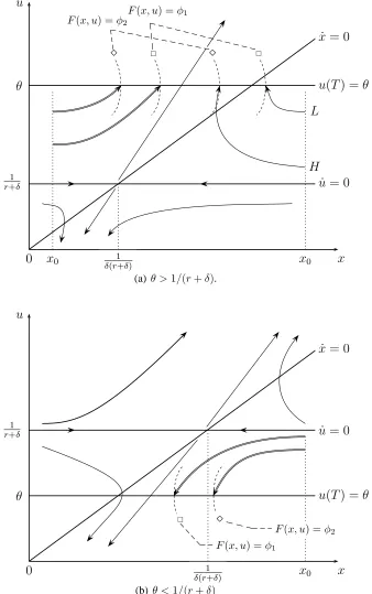
There are two possible configurations for the phase diagram corresponding to Eqs. (27a)-(27c). Figure 1(a) corresponds to the caseu(T)> uss, that is,θ >[r+δ]−1
, and Figure 1(b) to the caseu(T)< uss. In what follows, details pertaining to Figure 1(a) are given.
First, derive an explicit expression for the terminal value of the capital stock. Given that
u(T) =θfrom Eq. (27b), Eq. (27c) can be solved forx(T)to get
x(T) = φ−0.5θ
2
1−θ[r+δ]. (28)
The case of interest isx(T)>0, which is maintained in what ensues. Becauseu(T)> ussin the
present case, that is,θ >(r+δ)−1
, the denominator in Eq. (28) is negative, henceφ <0.5θ2. It
then follows that∂x(T)/∂φ = 1/[1−θ(r+δ)]<0, that is, an increase in the flow of sunk fixed costs decreases the capital stock the firm has on hand when it shuts down. Note that the opposite is true in Figure 1(b), whereu(T)< ussholds, in view of the fact thatθ <(r+δ)−1
u
x
˙
x= 0
˙
u= 0
1
r+δ
u(T) =θ θ
0 1
δ(r+δ)
x0 x0
L
H
⋄
⋄
F(x, u) =φ2
F(x, u) =φ1
(a)θ >1/(r+δ).
u
x
˙
x= 0
u(T) =θ θ
˙
u= 0
1
r+δ
0 1
δ(r+δ) x0
⋄
F(x, u) =φ2
F(x, u) =φ1
[image:21.595.142.480.127.666.2](b) θ <1/(r+δ)
F(x, u) =φin thexu-plane is given by:
∂u ∂x
Eq.
(27c)
= −Fx(x, u)
Fu(x, u)
F(x,u)=φ
= θ(r+δ)−1
θ−u
(
<0 iff u > θ
>0 iff u < θ , (29)
asθ(r+δ)−1> 0in the case under consideration. Eq.(29) also demonstrates that, asu →θ, the slope of the curve implicitly defined byF(x, u) =φbecomes vertical. As a result, the curve implicitly defined by the transversality condition F(x, u) = φ in Eq. (27c) and the horizontal straight line determined by the endpoint conditionu(T) =θ in Eq. (27b) intersect orthogonally at the optimal terminal time.
Finally, in order to complete the phase diagram, the curvature of the curve implicitly defined byF(x, u) =φmust also be determined. The said curvature is found by partially differentiating Eq. (29) with respect to u, remembering that u is a function of x alongF(x, u) = φ via the implicit function theorem:
∂2u ∂x2
F(x,u)=φ
= θ(r+δ)−1 [θ−u]2
∂u ∂x
F(x,u)=φ
(
<0 iff u > θ
>0 iff u < θ . (30)
Thus, under the present assumptions, Eqs. (29) and (30) show that the curve implicitly defined by
F(x, u) =φis increasing and strongly convex for all values ofubelowu(T) = θand decreasing and strongly concave for all values ofuaboveu(T) = θ.
Putting the above information together yields Figure 1(a), where the curvesF(x, u) =φand
u(T) = θ are shown intersecting in the northeast and northwest isosectors. Under the present stipulations, a solution to the adjustment cost problem must lie exclusively in the northwest isosector. To see this, recall that∂x(T)/∂φ = 1/[1−θ(r+δ)] <0. Thus, as the flow of sunk fixed costs increases, the point where the curvesF(x, u) = φandu(T) =θintersect moves to the left. Define two fixed costs,φ1andφ2, such thatφ2 > φ1. The preceding implies that, for paths originating in the northeast isosector of Figure 1(a), the trajectory corresponding toφ2, labeled
H, must lie below the trajectory corresponding to φ1, labeled L. Trajectory H therefore lies closer to the stable manifold of the saddlepoint steady state – theu˙ = 0isocline – implying that it has a larger value of terminal time than trajectoryL. Trajectories originating in the northeast isosector therefore exhibit the property that, as the flow of sunk fixed costs increases, the terminal time increases, which contradicts Proposition 4. As a result, a solution to problem (26) cannot originate in the northeast isosector, that is, it must lie exclusively in the northwest isosector.
double-lined trajectories correspond to the optimal time-paths of the capital stock and investment rate, and are monotonically increasing functions of time. They show that, the higher the flow of sunk fixed costs, the sooner the firm shuts down and the smaller is its capital stock when it does so.
Figure 1(b) shows the trajectories corresponding to a solution of the adjustment cost model whenu(T) < uss. By Proposition 4, it remains the case that the optimalT is lower when the
flow of sunk fixed costs are higher, but in this case the terminal stock of capital increases when the flow of sunk fixed costs increases, seeing as∂x(T)/∂φ = 1/[1−θ(r+δ)]>0. In contrast to the case of Figure 1(a), the capital stock and investment trajectories lie exclusively in the southeast isosector and are monotonically decreasing functions of time. Moreover, the analysis shows that, in general, the terminal stock of capital may increase or decrease as the flow of sunk fixed costs increases, thereby confirming that no general comparative statics result is available in Proposition 4 for the terminal value of the state vector.
5.2
Optimal pollution accumulation with uncertainty over the critical
pol-lution threshold
Tahvonen and Withagen (1996) developed a deterministic model of optimal pollution accumu-lation in which the pollution stock depreciates as long as it remains below a critical threshold. If the stock passes the threshold, it no longer depreciates and is therefore deemed to be ‘irre-versible’. The social planner is asserted to choose the rate of pollution-augmenting output over an infinite planning horizon that is divided into two distinct stages: during the first stage, the stock of pollution depreciates at a defined rate; during the second, upon reaching the threshold, the rate of depreciation falls to zero. One focus in the model is on the choice of the optimal timing of entry to the second stage.
function,U(·), in a general form. As a result, the planner solves:
max
y(·),T E0
Z T
0
U(y(t), z(t))e−ρt
dt+ (31a)
e−ρT
Z +∞
T
−1
2α2[z(t)]
2+β1y(t)− 1
2β2[y(t)]
2
e−ρ(t−T)dt
,
s. t. z˙(t) =y(t)−αz(t), z(0) =z0, z(T) =µZ+γZX, t∈[0, T], (31b)
˙
z(t) =y(t), t∈(T,+∞), (31c)
wherey(t)is the rate of pollution-augmenting output,z(t)the stock of pollution and the Greek letters are parameters, all of which are positive andX is a random variable with mean zero and variance 1. The pollution stock at which irreversibility occurs is therefore a random variable
z(T)from the perspective oft = 0, with meanµZ and varianceγZ2.
As in Tahvonen and Withagen, it is assumed that the planner knows the moment at which irreversibility occurs. Hence, at the point at which the second stage is entered, the planner solves the following deterministic control problem:
V2(zT) = max y(·)
Z +∞
T
−1
2α2[z(t)]
2 +β1y(t)− 1
2β2[y(t)]
2
e−ρ(t−T)dt, (32a)
s. t. z˙(t) =y(t), z(T) =zT
. (32b)
Noting that this is a deterministic version of problem (22), withα1 = 0,a= 0,b= 1andσ = 0, it follows from Proposition 6 that
V2(zT) =A[zT]2+BzT +C, (33)
whereA,B andCare as defined in Eq. (25).
From the perspective oft= 0, the planner solves:
max
y(·),T
Z T
0
U(y(t), z(t))e−ρt
dt
+e−ρT
E0[V2(z(T))], (34)
where, noting Eq. (33):
E0[V2(z(T))] =E0[A(µ2Z+ 2µZγZX+γZ2X2) +B(µZ+γZX) +C] =A(µ2Z+γZ2) (35)
+BµZ+C.
As the values of the stock of pollution are not decision variables at t = 0 and t = T, upon substituting E0[V2(Z(T))] for [S1(xT) +ψT] in Eq. (10a), it alone determines the optimal
value of T. Hence, implicitly differentiating the resulting Eq. (10a) with respect toγ2
Z yields
sign[∂T∗
/∂γ2
Z] = −sign[A]. Accordingly, for a risk averse planner,A < 0and it is optimal to
extend the first stage of the planning horizon, while if a planner is a risk lover, thenA >0and it is optimal to enter the risky second stage earlier.
5.3
A lifecycle model of retirement with shocks to retirement income
This section applies Proposition 5 to extend Prettner and Canning’s (2014) lifecycle model of retirement to establish the effect of idiosyncratic shocks to retirement income on the optimal timing of retirement. The defining characteristic of the analysis is that the solution of the retire-ment stage of the model yields a bequest function which is additive in the parameter governing the variance of the idiosyncratic shocks.
Consider, therefore, the following generalization of Prettner and Canning’s control problem, in which shocks to retirement income and a general utility function during working life are postulated:
max
c(·),l(·),WT,T
E0
Z T
0
U(c(t), l(t))e−ρt˜dt+e−ρT˜
Z +∞
T
ln[c(t)]e−ρ˜(t−T)dt
, (36a) s. t. W˙ (t) =wl(t) + ˜rW(t)−c(t), W(0) =W0, t∈[0, T], (36b) dW(t) = [rW(t)−c(t)]dt+σW(t)dZ(t), W(T) =WT, t ∈(T,+∞), (36c)
in a general form.
Inspection of problem (36a) shows that it is a special case of problem (17), whereα = 0, β = 1, a =randb =−1. It therefore follows from Proposition 5 that∂T∗
/∂σ2 >0, asα+β >0. That is, the presence of idiosyncratic shocks to retirement income unambiguously increases the optimal retirement age. The second stage shocks have the effect of introducing risk into the evolution of wealth during an agent’s retirement years, which the risk averse agent wishes to delay.
5.4
Further applications
In closing section 5, we briefly review several other papers in addition to those just discussed and those reviewed in sections 1 and 2, to which our results may be applied.
Consider first a pair of closely related papers by Caulkins et al. (2011, 2015). Each developed an optimal control model of conspicuous product pricing by a firm when an economy is in a recession that reduces demand and freezes credit markets, the latter extending the former by allowing the firm to develop an optimal cash management strategy. In the case when the recession lasts so long that the firm faces bankruptcy and therefore finds it optimal to shut down, the terminal time is a decision variable and hence Corollary 2 and Proposition 4 apply. As a result, in the case of an interior solution, a flow of sunk fixed costs affects the firm’s optimal price trajectory and, moreover, it will shut down sooner if the flow of sunk fixed costs increases. These results are intrinsic to the models, as they do not rely upon the functional form assumptions made by Caulkins et al. (2011, 2015).
Proposition 4 can also be used to show that an increase in a fixed switching cost delays the adoption decision in the Grass et al. (2012) two-stage optimal control model of technology adoption with capital accumulation and technological progress. Then either Proposition 5 or 6 can be used to extend the model to determine the effect of an increase in the instantaneous variance of the change in the post-adoption capital stock on the adoption decision when the second-stage control problem has an infinite planning horizon. Indeed, these three propositions can be applied just as readily to the two-stage optimal control models of workplace reorganization of Valle´e and Moreno-Galbis (2011) and closed- versus open-source software distribution of Caulkins et al. (2013), to draw similar qualitative conclusions.
the model, so Propositions 1-6 do not apply. But in discussing possible extensions of the model, Bultmann et al. (2008b) suggested that the switching time may be a decision variable as a result of a deliberate policy choice by a government, in which case Corollary 2 and Proposition 4 apply and Propositions 5 or 6 can be used to further extend the model and draw qualitative conclusions akin to those just mentioned.
With the growing use of two-stage optimal control problems to model all kinds of economic environments, as exemplified by Chapter 8 of Grass et al. (2008) and the applications contained therein, the number of papers which can take advantage of our basic results might be expected to increase in the coming years.
6
Concluding remarks
A framework for studying the impact of additive transformations to rewards for a general class of deterministic, nonautonomous optimal control problems has been established and a full set of comparative static results derived. The framework was then extended to two classes of stochas-tic control problems, one of which was the workhorse linear-quadrastochas-tic class. The reach of the methods was demonstrated on three rather different optimal control problems and an economic interpretation of the comparative statics calculations was provided.
When the planning horizon is fixed, neither the optimal time-paths of the control or state variables, nor the latter’s corresponding shadow prices, are functions of additive flow, start-up, or termination, sunk fixed costs or benefits. If, however, the initial or terminal time are decision variables – not uncommon in economic theory – then optimal time-paths of the state, control and costate variables, as well as the optimal initial and terminal times, are functions of additive flow and termination sunk fixed costs or benefits, but not such start-up costs and benefits.
Acknowledgements
We thank three anonymous referees and Associate Editor Mukerji for their suggestions on how to improve our paper. Remaining errors are our own.
References
Besanko, D. and Braeutigam, R. (2013). Microeconomics. Wiley, Hoboken, NJ, 5th edition.
Boucekkine, R., Pommeret, A., and Prieur, F. (2013). Optimal regime switching and threshold effects.
Journal of Economic Dynamics and Control, 37(12):2979–2997.
Boucekkine, R., Saglam, C., and Vale´e, T. (2004). Technology adoption under embodiment: a two-stage optimal control approach. Macroeconomic Dynamics, 8:250–271.
Bultmann, R., Caulkins, J., Feichtinger, G., and Tragler, G. (2008a). Modeling supply shocks in optimal control models of illicit drug consumption. In Lirkov, I., Margenov, S., and Wasniewski, J., editors,
Large-Scale Scientific Computing, volume 4818 of Lecture Notes in Computer Science, pages 285–
292. Springer Berlin Heidelberg.
Bultmann, R., Caulkins, J. P., Feichtinger, G., and Tragler, G. (2008b). How should policy respond to disruptions in markets for illegal drugs? Contemporary Drug Problems, 35:371–395.
Caputo, M. R. (2005). Foundations of Dynamic Economic Analysis: Optimal Control Theory and
Appli-cations. Cambridge University Press, Cambridge, First edition.
Caputo, M. R. and Wilen, J. E. (1995). Optimality conditions and comparative statics for horizon and endpoint choices in optimal control theory. Journal of Economic Dynamics and Control, 19:351– 369.
Caulkins, J. P., Feichtinger, G., Grass, D., Hartl, R. F., Kort, P. M., and Seidl, A. (2011). Optimal pricing of a conspicuous product during a recession that freezes capital markets. Journal of Economic
Dynamics and Control, 35:163–174.
Caulkins, J., Feichtinger, G., Grass, D., Hartl, R. F., Kort, P. M., and Seidl, A. (2013). When to make proprietary software open source. Journal of Economic Dynamics and Control, 37:1182–1194.
Caulkins, J., Feichtinger, G., Grass, D., Hartl, R. F., Kort, P. M., and Seidl, A. (2015). Capital stock management during a recession that freezes credit markets. Journal of Economic Behaviour &
Organization, 116:1–14.
Farmer, R. (1997). Intertemporal effects of environmental mandates. Environmental and Resource
Eco-nomics, 9:365–381.
Grass, D., Caulkins, J. P., Feichtinger, G., Tragler, G., and Behrens, D. A. (2008). Optimal Control of
Non-linear Processes: with Applications to Drugs, Corruption and Terror. Springer, Berlin Heidelberg,
Grass, D., Hartl, R., and Kort, P. (2012). Capital accumulation and embodied technical progress. Journal
of Optimization Theory and Applications, 154:588–614.
Lewis, T. R., Matthews, S. A., and Burness, H. S. (1979). Monopoly and the rate of extraction of ex-haustible resources. The American Economic Review, 69:227–230.
Makris, M. (2001). Necessary conditions for infinite-horizon discounted two-stage optimal control prob-lems. Journal of Economic Dynamics and Control, 25:1935–1950.
Prettner, K. and Canning, D. (2014). Increasing life expectancy and optimal retirement in general equilib-rium. Economic Theory, 56:191–217.
Quah, J. K.-H. and Strulovici, B. (2013). Discounting, values, and decisions. Journal of Political
Econ-omy, 121:896–939.
Rogerson, R. and Wallenius, J. (2013). Nonconvexities, retirement and the elasticity of labour supply. The
American Economic Review, 103:1445–1462.
Schmalensee, R. (1976). Resource exploitation theory and the behavior of the oil cartel. European
Economic Review, 7:257–279.
Seierstad, A. and Sydsæter, K. (1987). Optimal control theory with economic applications. North-Holland, Amsterdam, First edition.
Siebert, H. (1983). Extraction, fixed costs and the Hotelling Rule. Journal of Institutional and Theoretical
Economics, 139:259–268.
Tahvonen, O. and Withagen, C. (1996). Optimality of irreversible pollution accumulation. Journal of
Economic Dynamics and Control, 20:1775–1795.
Tomiyama, K. (1985). Two-stage optimal control problems and optimality conditions. Journal of
Eco-nomic Dynamics and Control, 9:317–337.
Valente, S. (2011). Endogenous growth, backstop technology adoption, and optimal jumps.
Macroeco-nomic Dynamics, 15:293–325.
Valle´e, T. and Moreno-Galbis, E. (2011). Optimal time switching from tayloristic to holistic workplace organization. Structural Change and Economic Dynamics, 22:238–246.
Appendix: Proofs of Propositions 5 and 6
Proof of Proposition 5. The first-order necessary condition of the maximization problem in
Eq. (19) givesu = −βb−1 [V′
2(x)]
−1
> 0, the strict inequality following from the fact that the domain of the natural logarithm function is(0,+∞). The second-order necessary condition is
−βu−2
≤ 0, which is equivalent toβ ≥ 0. But, seeing as β 6= 0 by assumption, it follows that
The supposition forV2(·)is given in Eq. (20), whereA, B, andC are constants to be deter-mined, and whereV′
2(x) =Ax
−1
+BandV′′
2 (x) =−Ax
−2
. Substitutingu=−βb−1 [V′
2(x)]
−1
>
0and the expressions forV2(x), V′
2(x)andV
′′
2 (x)in Eq. (19) gives rAlnx+rBx+rC =αlnx+βln[−b−1
β[Ax−1
+B]−1
] +aBx+aA−β− 1
2σ
2A. (37)
Equating coefficients on like terms in Eq. (37) results in
A =r−1
(α+β), (38a)
B = 0, (38b)
C =r−1
β[ln(−b−1
rβ(α+β)−1
)−1] +r−2
(α+β)
a− 1
2σ
2
, (38c)
as the values of the three constants such that Eq. (20) is the stage two current value function. Now observe thatu = −βb−1
[V′
2(x)]
−1
= −βb−1
r(α+β)−1
x > 0, which is equivalent to
b(α+β)<0, because none of the terms in the product can be zero andx >0,β > 0andr >0. Finally, in order to prove thatsign[∂T∗
/∂σ2] =sign[α+β], first recall that the initial state
variable is not a decision variable and the terminal state is a scalar. Upon settingS1(x
T) +ψT =
V2(xT)and using Eq. (38), it follows that Eqs. (10a) and (10c) implicitly yield the optimal values
of (T, xT). It then follows from differentiating the identity form of Eqs. (10a) and (10c) with
respect toσ2 that:
H∗
∂T∗
(β)/∂σ2 ∂x∗
T(β)/∂σ2
≡
−12r−1
e−rT(α+β)
0
, (39)
and therefore that∂T∗
(β)/∂σ2 ≡ −1 2r
−1
e−rT(α+β)( ˆV
xTxT +e −rTS1
xTxT)/|H ∗
|. Given the second-order sufficient conditions, the result sign[∂T∗
/∂σ2] = sign[α+β]is immediate. Q.E.D.
Proof of Proposition 6. The first-order necessary condition of the maximization problem in
Eq. (22) is equivalent tou= β−1
2 [β1 +bV
′
2(x)] ≥ 0, the inequality following from the fact that
the control variable is constrained to be nonnegative. The second-order necessary condition is
−β2 ≤ 0, which is equivalent to β2 ≥ 0. But seeing asβ2 6= 0 by assumption, it follows that
β2 >0.
Substitutingu=β−1
2 (β1+bV
′
2(x))and the expressions forV2(x),V
′
2(x)andV
′′
2 (x)into Eq.
(23), yields: 1
2rAx
2+rBx+rC =
aA+ 1 2b
2β−1
2 A2−
1 2α2
x2+ (α1+aB+b2β−1
2 AB+bβ1β
−1
2 A)x
(40) + 1 2β 2 1β −1 2 + 1 2b
2β−1
2 B2+bβ1β
−1
2 B+
1 2σ
2A
.
Equating coefficients on like terms in Eq. (40) yields the solutions for A, B, and C given in Proposition 6. Recalling thatu=β−1
2 (β1+bV
′
β1+bV′
2(x) =β1+bB+bAx≥0.
Finally, repeating the steps that led to Eq. (39):
H∗
∂T∗
(β)/∂σ2 ∂x∗
T(β)/∂σ2
≡
1
2e
−rTA
0
,
and therefore that∂T∗
(β)/∂σ2 ≡ 1 2e
−rTA( ˆV
xTxT +e−rTSx1TxT)/|H ∗
|. Given the second-order sufficient conditions, the result sign[∂T∗