The a-function for gauge theories

LTH1017

The

a

-function for gauge theories

I. Jack1 _{and C. Poole}2

Dept. of Mathematical Sciences, University of Liverpool, Liverpool L69 3BX, UK

Abstract

The a-function is a proposed quantity defined for quantum field theories which has a monotonic behaviour along renormalisation group flows, being related to the

β-functions via a gradient flow equation involving a positive definite metric. We construct thea-function at four-loop order for a general gauge theory with fermions and scalars, using only one and two loop β-functions; we are then able to provide a stringent consistency check on the general three-loop gauge β-function. In the case of an N = 1 supersymmetric gauge theory, we present a general condition on the chiral field anomalous dimension which guarantees an exact all-orders expression for thea-function; and we verify this up to fifth order (corresponding to the three-loop anomalous dimension).

1_{dij@liv.ac.uk}

1

Introduction

It is natural to regard quantum field theories as points on a manifold with the couplings

{gI} as co-ordinates, and with a natural flow determined by the β-functions βI(g). At fixed points the quantum field theory is scale-invariant and is expected to become a con-formal field theory. It was suggested by Cardy [1] that there might be a four-dimensional generalisation of Zamolodchikov’s c-theorem [2] in two dimensions, such that there is a functiona(g) which has monotonic behaviour under renormalisation-group (RG) flow (the strong a-theorem) or which is defined at fixed points such that aUV−aIR >0 (the weak

a-theorem). It soon became clear that the coefficient (which we shall denote 1₄A) of the Gauss-Bonnet term in the trace of the energy-momentum tensor is the only natural candi-date for thea-function. A proof of the weaka-theorem has been presented by Komargodski and Schwimmer [3] and further analysed and extended in Refs. [4, 5].

In other work, a perturbative version of the strong a-theorem has been derived [6] from Wess-Zumino consistency conditions for the response of the theory defined on curved spacetime, and with x-dependent couplings gI(x), to a Weyl rescaling of the metric [7]. This approach has been extended to other dimensions in Refs. [8, 9]. The essential result is that we can define a function ˜A by

˜

A=A+WIβI, (1.1)

whereAis defined above andWI is well-defined as an RG quantity on the theory extended

as described above, such that ˜A satisfies the crucial equation

∂IA˜=TIJβJ, (1.2)

for

TIJ =GIJ + 2∂[IWJ]+ 2 ˜ρ[I ·QJ]. (1.3) HereGIJ =GJ I, ˜ρIandQJ may all be computed perturbatively within the theory extended

to curved spacetime and x-dependent gI_{; for weak couplings G}

IJ can be shown to be

positive definite in four dimensions (in six dimensions,GIJ has recently been computed to

be negative definite at leading order [10]). Eq. (1.2) implies

µ d dµ

˜

A=βI ∂

∂gIA˜=GIJβ

I_βJ _(1.4)

thus verifying the strong a-theorem so long as GIJ is positive. Crucially Eq. (1.2) also

imposes integrability conditions which constrain the form of the β-functions and are the focus of this paper. These conditions relate contributions to β-functions at different loop orders.

We should mention here that for theories with a global symmetry,βI in these equations should be replaced by aBI _{which is defined, for instance, in Ref. [6]; however it was shown}

that there is no difference to all orders in supersymmetric theories (see Ref. [14] for related results). Hence for our purposes in this article we may ignore the distinction.

The analysis of Ref. [6] was recently further extended in Ref. [15] (related results were also presented in Ref. [16]). Expressions for the three-loop Yukawaβ-functions and for the three-loop contribution to the metricGIJ were derived for a general fermion-scalar theory,

and Eq. (1.2) was checked up to this order; indeed it was shown that Eq. (1.2) places strong constraints upon the form of the β-function at this order. The N = 1 supersymmetric Wess-Zumino model was also considered as a special case. Moreover, here it was possible to show that an exact formula for the a-function conjectured in Refs. [17–19] was valid at this order; in previous work [20] this had been checked at the level of the two-loop β -functions for a general, gaugedN = 1 supersymmetric theory (in the rest of this paper we shall describe this as a “two-loop check” although the correspondinga-function is actually a four-loop quantity). A sufficient condition on the chiral field anomalous dimension for this exact a-function to be viable was presented and shown (using the results of Ref. [21, 22]) to be satisfied up to three loops for the Wess-Zumino model.

Our goal in this article is to extend the work of Ref. [15] to the gauge case. In the non-supersymmetric case, we show that the two-loop Yukawa β-function for the most general renormalisable gauge theory coupled to fermions and scalars is compatible with Eq. (1.2); indeed by imposing Eq. (1.2) we are able to obtain the terms in ˜A containing scalar or Yukawa couplings at this order up to only three free parameters, without any further perturbative calculations–this approach has previously been applied in Ref. [23] to the case of the standard model. (Of course a gradient flow for purely scalar quantum field theories was postulated some time ago by Wallace and Zia [24].) As a bonus, we show that this expression for ˜A is also consistent with (and provides a stringent check upon) the generalthree-loop gauge β-function derived by Gracey, Jones and Pickering [25]. As a further check, we also compute ˜A using the dimensional reduction version of the Yukawa

β-function and show that in the supersymmetric case, this reduces to the version of ˜A

presented in Ref. [20] (and is hence compatible with Ref. [17–19]). Finally, again in the context of supersymmetry, we extend the condition on the chiral superfield anomalous dimension presented in Ref. [15] to the gauge case and show that it is satisfied at three loops. We also derive the (very non-trivial) constraints that this condition imposes upon the form of the three-loop anomalous dimension.

2

The non-supersymmetric case

We consider a general renormalisable gauge theory with a simple gauge group G and nϕ

real scalars ϕa, nψ two-component Weyl fermions ψi, where G ⊂ U(nψ)∩O(nϕ). For a

Yukawa interaction 1₂ψiTC(Ya)ijψjϕa+h.c. and a quartic scalar interaction_4!1λabcdϕaϕbϕcϕd

and with a gauge coupling g the basic couplings are then

The (hermitian) gauge generators for the scalar and fermion fields are denoted respectively

tϕ_A =−tϕ_AT _{and t}ψ

A, A= 1. . . nV, wherenV = dimG, and obey

[tA, tB] =ifABCtC, (2.2)

and gauge invariance requires YatψA+t ψ

AT Ya =tϕAabYb,tϕAaeλebcdϕaϕbϕcϕd= 0. In order to

simplify the form of our results, it is convenient to assemble the Yukawa couplings into a matrix

ya=

Ya 0

0 Y¯a

, yˆa=

_¯

Ya 0

0 Ya

=σ1yaσ1, (2.3) and

TA=

tψ_A 0 0 −tψ_A∗

, TˆA=σ1TAσ1 =−TAT . (2.4)

This corresponds to using the Majorana spinor Ψ =

ψi

−C−1ψ¯iT

.

We should mention here that in our present calculations we have ignored potential parity violating counterterms (i.e. containing -tensors). The analysis of Ref. [6] was recently extended [28] to the case of theories with chiral anomalies, including the possibility of parity violating anomalies. It would be interesting to carry out the detailed computations necessary to exemplify the general conclusions of Ref. [28].

The one- and two-loop gauge β-functions are given by

βg =−β0g3−β1g5−g3 1 2nV

tr[Cψyˆaya],

β0 = 1₃(11CG−2Rψ− 1₂Rϕ),

β1 = 1₃CG(34CG−10Rψ−Rϕ)−

1

nV

tr[(Cψ)2]− 4 nV

tr[(Cϕ)2], (2.5) where

tr[tψ_Atψ_B] =RψδAB, tr[tϕ_Atϕ_B] =RϕδAB,

Cϕ =tϕ_Atϕ_A, Cψ =TATA, Cˆψ =Cψ T , (2.6)

with TA as defined in Eq. (2.4). We follow Ref. [15] in removing factors of 1/16π2 which

arise at each loop order by redefining

λabcd →16π2λabcd, Ya→4πYa, g →4πg . (2.7)

The one-loop Yukawa β-function is given by

β_{y a}(1) = 2ybyˆayb+1₂[ybyˆb−6g2Cˆψ]ya+1₂ya[ˆybyb−6g2Cψ] +1₂ tr[yayˆb]yb, (2.8)

and the one-loop scalar β-function is given by 1

4!β (1)

λ abcdϕaϕbϕcϕd=

1

8λabefλcdef + 3 2 g

4

(tϕ_Atϕ_B)ab(tϕ_Atϕ_B)cd− 1₂tr[yayˆbycyˆd]

− 1 2λabceg

2_(Cϕ₎

ed+ ₁₂1 λabcetr[yeyˆd]

The leading terms in the metric GIJ in Eq. (1.2) may be written as [6]

ds2 =GIJdgIdgJ = 2nV

1

g2(1 +σg

2_)(dg)2₊ 1

6tr[dˆyadya] + 1

144dλabcddλabcd, (2.10) where σ is given (using dimensional regularisation, DREG) by [6, 20]

σ = 1₆ 102CG−20Rψ −7Rϕ

. (2.11)

We emphasise here that y and ˆy are not independent; and furthermore, the result of a trace is unchanged by interchanging y and ˆy.

The lowest-order contributions to ˜A are given implicitly in Ref. [20] as ˜

A(2) =−nVβ0g2, ˜

A(3) =− 1 2nVg

4

(β1+σ β0)−1₂g2tr[yayˆaCˆψ]

+ ₂₄1 (tr[yayˆaybyˆb] + 2 tr[yayˆbyayˆb] + tr[yayˆb] tr[yayˆb]). (2.12)

They can easily be checked to satisfy Eq. (1.2) with Eqs. (2.5), (2.8).

To proceed to the next order, we shall need the two-loop Yukawaβ-function in addition to the one-loop scalar β-function in Eq. (2.9). The two-loop β-function is given in general by Refs. [26, 27] in the form

β_{y a}(2) = 7

X

α=1

cα(Gyα)a+

19

X

α=8

cα[(Gyα)a+ ( ˆGyα)a)

+c20g4( ˆCψya+yaCψ) +c21g4CˆψyaCψ

+c22g4[( ˆCψ)2ya+ya(Cψ)2] +c23g4(Cϕ)ab( ˆCψyb +ybCψ)

+ tr[c24yayˆbycyˆc+c25yayˆcybyˆc+c26g2Cˆψyayˆb]

+c27g4(Cϕ2)ab+c28g4(Cϕ)ab+c29λacdeλbcde

yb. (2.13)

The contributions Gy

α are depicted in Table (1); ˆGyα is the transpose of Gyα. A solid or

open box represents g2Cψ or g2Cϕ respectively. A box with a letter “A” represents the gauge generator gTA. Note that for each of Gyα, there is an alternation between “hatted”

and “unhatted” y matrices, as can be seen in Eq. (2.13) for Gy

α, α = 20, . . .28. To give a

couple of examples, Gy₄ represents

(Gy₄)a =λabcdybyˆcyd, (2.14)

and Gy₁₉ corresponds to

Gy₁ Gy₂ Gy₃ Gy₄

Gy₅ Gy₆ Gy₇ Gy₈

Gy₉ Gy₁₀ Gy₁₁ Gy₁₂

A A

Gy₁₃ Gy₁₄ Gy₁₅ Gy₁₆

Gy₁₇ Gy₁₈ Gy₁₉

Table 1: The diagrams contributing to βy a(2)

We present here the results for the coefficients evaluated using standard dimensional regularisation, DREG [26, 27]:

c1 = 2, c2 =−1, c3 =−2, c4 =−2, c5 =−12,

c6 = 6, c7 = 0, c8 =−1₈, c9 = 0, c10 =−3₈, c11 =−1,

c12= 0, c13 =−7₄, c14 =−₄1, c15 = 6, c16 = 9₂, c17 = 0,

c18= 3, c19 = 5, c20 =−₁₂1 194CG−20Rψ −11Rϕ

, c21= 0, c22 =−3₂, c23 = 6, c24 =−3₄, c25 =−1₂,

have the freedom to redefine the couplings, corresponding to a change in renormalisation scheme; at this order we may consider

δya =µ1ybyˆayb+µ2(ybyˆbya+yayˆbyb) +µ3tr[yayˆb]yb

+µ4g2( ˆCψya+yaCψ) +µ5g2Cabφyb,

δg = (ν1CG+ν2Rψ+ν3Rφ)g3. (2.17) This results in a change in the β-function

δβ_{y a}(2) =

β_y(1)· ∂ ∂y +β

(1)

g

∂ ∂g

δya−

δy· ∂ ∂y +δg

∂ ∂g

β_{y a}(1). (2.18) Using Eqs. (2.5), (2.8) this leads to

δc2 =µ1−4µ3, δc6 =−4µ5, δc7 =−µ5, δc9 =−µ1+ 4µ2,

δc10=µ2−µ3, δc11=µ1−4µ2, δc13 =−6µ2−µ4, δc14=−6µ2−µ4,

δc16=−µ5, δc19=−6µ1−4µ4, δc24 =−2µ2+ 2µ3, δc25 =−µ1+ 4µ3,

δc26= −12µ3−2µ4,

δc20= 2CG 3ν1− 11₃ µ4

+ 2Rψ 3ν2+2₃µ4

+Rφ 6ν3+ 1₃µ4

,

δc28= −1₃ 22CG−4Rψ−Rφ

µ5. (2.19)

We observe that the redefinitions corresponding to µ1−4 are not all independent; for in-stance we may remove µ4 by redefining

µ1 →µ1− 2₃µ4, µ2 →µ2 −1₆µ4, µ3 →µ3−1₆µ4,

ν1 →ν1+ 11₉µ4, ν2 →ν2−2₉µ4, ν3 →ν3− ₁₈1µ4, (2.20) This is a general consequence of the form of the redefinition given by Eq. (2.18), which implies that a redefinition

δya =βy a(1), δg =β

(1)

g (2.21)

has no effect on βy a(2); however µ5 yields an independent redefinition due to the fact that there happens to be no corresponding C_abφyb term in β

(1)

y a. It then follows that µ1−5 and

ν1−3 yield only 7 independent redefinitions; we therefore have 33 −7 = 26 independent coefficients in the two-loop β-function. Under the change Eq. (2.17)

δA˜(3) =−δg ∂ ∂g

˜

A(2), (2.22)

which corresponds to taking δσ = 4 ν1CG+ν2Rψ+ν3Rφ

in Eq. (2.10). Applying Eq. (1.2), we require ˜A(4) _{to satisfy}

dyA˜(4) = dy·Tyy(3)·β

(1)

y +t1gtr[dˆyayaCψ]βg(1)+t2g(Cϕ)abtr[dˆyayb]βg(1)

+ 1

12tr[dˆyaβ (2)

y a],

dλA˜(4) = ₁₄₄1 dλabcdβ

(1)

GT₁ GT₂ GT₃ GT₄

GT₅ GT₆ GT₇ GT₈

GT₉ GT₁₀

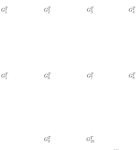
Table 2: Contributions to dy·Tyy(3)·d0y

where dy = dy·_∂y∂, etc, the lower-order metric contributions were read off from Eq. (2.10)

and we write

dy·T_yy(3)·d0y= 10

X

α=1

TαGTα, (2.24)

The contributions to dy ·Tyy(3) · d0y at this order are depicted in Table (2). Here a

diamond represents d0y and a cross dy. As an example,GT

1 represents

GT₁ = tr[dˆyaybyˆbd0ya]. (2.25)

Tyy(3) is symmetric up to the order at which we are working. The β-functions βg(1), βy(1)

in Eq. (2.23) are given in Eqs. (2.5), (2.8). There are no “off-diagonal” fermion-scalar contributions to this order. We parameterise ˜A(4) _as

˜

A(4)= 28

X

α=1

AαGAα + O(g

6

), (2.26)

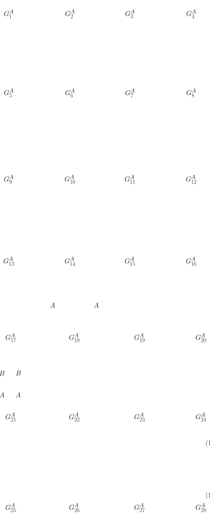
where the different contributions GA

α are depicted in Table (3), with a similar notation to

Table (2). We have includedGA

28 as a reflection of the general freedom to redefine ˜

GA₁ GA₂ GA₃ GA₄

GA

5 GA6 GA7 GA8

GA₉ GA₁₀ GA₁₁ GA₁₂

GA₁₃ GA₁₄ GA₁₅ GA₁₆

A A

GA₁₇ GA₁₈ GA₁₉ GA₂₀

B

A A B

GA₂₁ GA₂₂ GA₂₃ GA₂₄

(1)y

(1)y GA₂₅ GA₂₆ GA₂₇ GA₂₈

together with a related redefinition of TIJ; see Ref. [15] for further details. The purely g

-dependent contributions to ˜A(4)_{of course cannot be determined from Eq. (2.23). Eq. (2.23)} entails the system of equations

6A4 = 1₆c1, 2A11+ 4A28= 1₂T8+ ₆1c2 = 2T6+ 2T5+ ₆1c25 = 2T4+1₂T7,

2A10+ 8A28= 2T7+ ₆1c3 =T8, 4A3 = 1₆c4, 2A17 = 2T10+ 1₆c5 = 1₆c6, 4A20 = 1₂T10+ 1₆c7, 4A6+ 2A28 = 1₂(T2+T3) + 1₃c8 =T1, 2A9+ 8A28 = 2T2+ 2T3+ 1₃c9 =T7+1₂T8+1₃c11= 2T1+1₂T8,

2A7+ 2A28= 1₂(T2+T3) + 1₃c10 = 1₂T1+T4 =T6+T5+1₆c24, 2A14−12A28=−3T1+ 1₂T9+ 1₃c12 =−3T2−3T3+ 1₃c14,

4A13−24A28=−3(T1+T2+T3) + 1₂T9+1₃c13, 4A18= 1₃c15, 2A15 = 1₃c16=T10+1₃c17, 2A16−48A28= 2T9−3T8+ 1₃c18 =−6T7−3T8+ 1₃c19, 2A26 = 1₃c20,

36A28+ 2A23 =−3T9+ 1₆c21, 36A28+ 2A22 =−3T9+ 1₃c22, 2A25 =−6T10+1₃c23, 2A19−12A28=−6T6−6T5+ 1₆c26 =−6T4+ 1₂T9,

2A24= 1₆c27, 2A27 = 1₆c28, 2A2 = 1₆c29,

6A5+ 3A28 = 1₂(T1 +T2 +T3), 6A8+3₂A28= 1₂(T4+T6+T5) (2.28) where the cα are given in Eq. (2.16). (The coefficients A1, A12 and A21 are determined immediately by the second of Eqs. (2.23), so we simply list their values later in Eqs. (2.31).) Solving Eqs. (2.28), we find the conditions

T2+T3 = 2T1− 2₃c8, T4 = 1₂T1− 1₃c8+1₃c10,

T5+T6 =T1−1₆c24−1₃c8+1₃c10, T7 = 2T1− 1₃c11,

T8 = 4T1− 8₃c8+2₃c9, T9 =−6T1 + 2c24+1₃c26, T10 = ₁₂1 (c6−c5), (2.29) together with conditions on the β-function coefficients

c2 =−1₄c3−c9+ 4c10, c11= 1₄c3+ 4c8 −c9,

c5−c6 =−4(c16−c17), c14= 3₈c3− 3₂c9+c12−1₄(c18−c19)

c24= 1₈c3+ 2c8−1₂c9+ 1₂c25, c26=−1₂(c18−c19)−3c25. (2.30) The conditions on T1−6 in Eq. (2.29) were already derived in Ref. [15]. Reassuringly, the conditions Eq. (2.30) are satisfied by the coefficients in Eq. (2.16), and also by the redefi-nitions in Eq. (2.19). These six constraints in principle leave only 19 of the 25 independent coefficients in the two-loop β-function to be determined by perturbative computation.

A1 = ₁₄₄1 , A2 = ₁₄₄1 , A3 =−₁₂1, A4 = ₁₈1 , A5 = ₁₄₄1 , A6 =A11= 0,

A7 =−₂₄1, A8 =−₂₈₈1 , A9 = ₁₂1, A10= 1₆, A12 =−₂₄1, A13=−₂₄7,

A14=−1₆, A15 = 3₄, A16=−2₃, A17= 1₂, A18 = 1₂, A19= ₁₂1,

A20 = ₁₆3 , A21 = 1₄, A22= 3₄, A23= 1, A24=−₈7, A25=−7₂,

A26 =−₇₂1 (194CG−20Rψ −11Rϕ)−t1β0,

A27 = ₁₄₄1 (147CG−12Rψ −3Rϕ)−t2β0, (2.31) where β0 is given in Eq. (2.5). Since A6 only appears in Eq. (2.28) in the combination 4A6+ 2A28, we have setA6 = 0 in line with Ref. [15]. We note that under the redefinitions in Eq. (2.17),

δA˜(4) =−

δy· ∂

∂y +δg ∂ ∂g

˜

A(3)+ O(g6). (2.32) Moreover the effect of these redefinitions on the metric coefficients in Eq. (2.23) (as parametrised in Eq. (2.24)) may easily be computed using Eq. (2.10) as

δT1 =δT2 =δT3 =−2₃µ2,

δT4 =δT5 =δT6 =−1₃µ3,

δT7 =1₂δT8 =−1₃µ1,

δT9 =−2₃µ4, δT10=−1₃µ5,

δt1 =−4₃µ4, δt2 =−2₃µ5. (2.33) Using Eq. (2.19)), these results are easily seen to agree with Eq. (2.29).

It is remarkable that no knowledge of the “metric” coefficients Tα is required to

deter-mine the Aα in this fashion; of course the ti in Eq. (2.31), which define the “off-diagonal”

fermion-gauge metric in Eq. (2.23), could be determined by a perturbative calculation if required, as was accomplished for the fermion-scalar case in Ref. [15]. The results in Eq. (2.31) will be used in Sect. 3 in a check of the three-loop βg.

In Ref. [15] the extension to three loops was accomplished by first inferring the three-loop Yukawa β-function for a chiral fermion-scalar theory, using the three-loop results de-rived in Ref. [30] for the standard model, combined with the results for the supersymmetric Wess-Zumino model. Such an approach will not work in the gauged case, unfortunately; the results of Ref. [30] are only for the SU(3) colour gauge group, which of course is not sufficient to determine how the three-loop Yukawa β-function depends on a general gauge coupling.

3

The three-loop gauge

β

-function

compatible with this result via Eq. (1.2). In fact, our result for ˜A(4) determines the 16 terms inβg(3)with Yukawa couplings up to 4 (see later) unknown parameters. It is rather striking

that the two-loop calculation of βy(2) (and the one-loop result β_λ(1)) have thereby provided

so much information on a three-loop RG quantity. This is an example of the “3−2−1” phenomenon noted in Refs. [23, 31]; namely that the gauge-gauge, fermion-fermion and scalar-scalar contributions to the metric GIJ start at successive loop orders.

In our notation, βg(3) can be written

1

gβ

(3)

g =

1 16nV −

2 3G

A

12+G

A

13+ 3G

A

14+ 4G

A

15+ 12G

A

16−8G

A

17+ 8G

A

18 + 7GA₁₉−GA₂₀+ 8G₂₁A −10GA₂₂−2GA₂₃

−28GA₂₄−64GA₂₅−48CGGA26+ 18CGGA27+ O(g 6₎

, (3.1)

where the GA

α are implicitly defined in Table (3). The purely g-dependent terms are not

determined in this analysis. It is then easy to show, using Eqs. (2.26), (2.31), that we can write

g ∂ ∂g

˜

A(4) =T_gg(1)β_g(3)+T_gg(2)β_g(2)+T_gg(3)β_g(1)+T_gy(3)·β_y(1), (3.2) in the form,

g ∂ ∂g

˜

A(4)= 2nV 1_gβg(3)+

1

3gnV 102CG−20R

ψ _−7Rϕ

β_g(2)+T_gg(3)β_g(1) −g2 17₁₂tr[ˆyaCϕβy a(1)] +g

2_(Cϕ₎

abtr[ˆyaβ

(1)

y b], (3.3)

where βg(1), βg(2) are given in Eq. (2.5). We notice that Tgg(2) agrees with the result for σ in

Eq. (2.11). Tgg(3) takes the form

T_gg(3) =g −10 3 + 4t1

tr[ˆyayaCψ] +g −1₂ + 4t2

(Cϕ)abtr[yayˆb] + O(g3). (3.4)

Unfortunately we have no means of disentangling the separate purely g-dependent contri-butions in ˜A4 _{and in T}(3)

gg βg(1), without a three-loop calculation; but all the Yukawa or λ

dependent contributions match exactly. If

t1 =−17₁₂, t2 = 1, (3.5)

then we would haveTIJ symmetric at this order; but as demonstrated in Ref. [15], at three

loops TIJ is not symmetric even for a pure fermion-scalar theory for a general

renormali-sation scheme.

Had we not knownβg(3) then it would have been determined by Eq. (3.2) up to the four

parameters consisting of the two coefficients in Tgy(2) and the two coefficients in Tgg(3) (the

4

The supersymmetric case

Here the analysis is extended to a generalN = 1 supersymmetric gauge theory, which may in principle be obtained from the general non-supersymmetric theory discussed in Sect. 2 by an appropriate choice of fields and couplings. Such a theory can of course be rewrit-ten in terms of nC chiral and corresponding conjugate anti-chiral superfields, and indeed

perturbative computations are enormously simplified through the use of this formalism; moreover, in the light of the non-renormalisation theorem and the NSVZ formula [32, 33] for the exact gauge β-function, the renormalisation of the theory is essentially entirely determined by the chiral superfield anomalous dimension γ (at least in a suitable renor-malisation scheme). In this section we shall therefore start anew using results derived using superfield methods. Nevertheless, in Sect 5 we show that (at least up two loops) the results obtained using the two approaches match, as indeed they must.

The crucial new feature in the supersymmetric context is the existence of a proposed exact formula for the a-function [17–19]. This exact form was verified up to two loops in Ref. [20] for a general supersymmetric gauge theory, and up to three loops [15] in the case of the Wess-Zumino model. Moreover in Ref. [15] a sufficient condition on γ to guarantee the validity of this exact result was found and shown to be satisfied up to three loops; related considerations appear in Refs. [18, 19], see later for a discussion. In this section we shall generalise this condition to the gauged case and check that it is satisfied up to three loops, using the results of Ref. [22].

The couplings gI are now given by gI = {g, Yijk,Y¯ijk} with ¯Yijk = (Yijk)∗. The

supersymmetric Yukawa β-functions are expressible in terms of the anomalous dimension matrix γij in the form

βY =Y ∗γ , β_Y¯ =γ∗Y ,¯ (4.1)

where for arbitrary ωij we define

(Y ∗ω)ijk ≡Yljkωli +Yilkωlj+Yijlωlk,

(ω∗Y¯)ijk ≡ωilY¯ljk+ωjlY¯ilk+ωklY¯ijl. (4.2)

We also introduce a scalar product for Yukawa couplings3

Y ◦Y¯ = ¯Y ◦Y = 1

6Y

ijk_Y¯

ijk, (4.3)

and it is further useful to define

( ¯Y Y)ij = 1₂Y¯iklYjkl ⇒ Y ◦(ω∗Y¯) = (Y ∗ω)◦Y¯ = tr ( ¯Y Y)ω. (4.4)

The gauge β-function is assumed to have the form

βg =f(g) ˜βg, β˜g =Q−2nV−1tr[γ CR], f(g) =g3+ O(g5), (4.5)

where, with RA the gauge group generators,

Q=TR−3CG, TRδAB = tr(RARB), CGδAB =fACDfBCD, (CR)ij = (RARA)ij,

(4.6) and nV is the dimension of the gauge group. For gauge invariance we must have

Y ∗RA= 0, RA∗Y¯ = 0. (4.7)

Under a change g →g0(g) = g+ O(g3_{) then in Eq. (4.5)}

f(g)→f0(g0) = ∂g

0

∂g f(g), γ(g)→γ

0

(g0) = γ(g), (4.8) assuming g0 is independent ofY,Y¯. For an infinitesimal change δf =f ∂gδg−δg ∂gf and

δγ =−δg ∂gγ. The NSVZ form for the β-function is obtained if

f(g) = g 3

1−2CGg2

. (4.9)

The resulting expression forβg originally appeared (for the special case of no chiral

super-fields) in Ref. [29], and was subsequently generalised, using instanton calculus, in Ref. [32]. (See also Ref. [33].) We note here that this result (called the NSVZ form ofβg) is only valid

in a specific renormalisation scheme, which we correspondingly term the NSVZ scheme. The exact expression generalises one and two-loop results obtained in Refs. [34–36]. These results were computed using the dimensional reduction (DRED) scheme; though in any case, the DRED and NSVZ schemes only part company at three loops [39].

The one and two-loop results for γ are given by [37, 38]

γ(1) =P ,

γ(2) = −S1 −2g2CRP + 2g4Q CR, (4.10)

where P and S1 are defined by

Pij = ( ¯Y Y)ij −2g2(CR)ij,

S1ij = ¯YiknYjmnPmk. (4.11)

We use here the notation and conventions of Ref. [22].

In the supersymmetric theory Eq. (1.2) is assumed to now take the form dYA˜= 1₂dY ◦TYY¯ ◦β_Y¯ + dY ◦T_{Y g}β˜_g,

dgA˜= dg Tggβ˜g +TgY ◦βY +TgY¯ ◦β_Y¯, (4.12) (with a similar equation for d_Y¯A˜). We have written the RHS in terms of ˜βg, effectively

the first of Eqs (4.12) since are not necessary to the order we shall consider. For N = 1 supersymmetric theories there is, at critical points with vanishing β-functions, an exact expression for a [17] in terms of the anomalous dimension matrix γ or alternatively the

R-charge R = 2₃(1 +γ). Introducing terms linear in β-functions there is a corresponding expression which is valid away from critical points and this can then be shown to satisfy many of the properties associated with thea-theorem [18], [19]. For the theory considered here, with nC chiral scalar multiplets, these results take the form

˜

A= ₁₂1 (nC + 9nV)− 1₂tr(γ2) + 1₃tr(γ3) + Λ◦β_Y¯ +n_V λβ˜_g+β_Y ◦H◦β_Y¯ , (4.13)

where ˜βg is given by Eq. (4.5) and we require

Λ◦β_Y¯ =β_Y ◦Λ¯. (4.14)

For the remainder of this section we omit for simplicity the term involvingH in Eq. (4.13); but return to it in Sect. 5. In Refs. [18] and [19] Λ, λ are Lagrange multipliers enforcing constraints on the R-charges. At lowest order the result for Λ and also the metric G

obtained in Ref. [18] are equivalent, up to matters of definition and normalisation, with those obtained here. The general form for ˜A given by Eq. (4.13) was verified up to two-loop order (for the anomalous dimension) in Ref. [20]. Λ may be constrained by imposing Eq. (4.12). Then

dYA˜= tr

dYγ ( ¯YΛ)−2λ CR−γ+γ2

+ (dYΛ)◦β_Y¯ +nV dYλβ˜g. (4.15)

We also have

dgA˜= tr

dgγ ( ¯YΛ)−2λ CR−γ+γ2

+ (dgΛ)◦β_Y¯ +nV dgλβ˜g. (4.16)

Hence if Λ, λ are required to obey

( ¯YΛ)−2λ CR =γ−γ2+ Θ◦β_Y¯ +θβ˜g, (4.17)

where making the indices explicit Θ◦d ¯Y → Θ_ij,klmd ¯Y_klm and θ → θ_ij, Eq. (4.13) then

satisfies Eq. (4.12) if we take 1

2dY◦TYY¯ ◦d ¯Y = tr

dYγ Θ◦d ¯Y

+ dYΛ◦d ¯Y ,

dY ◦T_{Y g} = tr[d_Yγ θ] +n_V d_Yλ ,

dg Tgg = tr [dgγ θ] +nV dgλ ,

dg TgY¯ ◦dY¯ = tr

dgγΘ◦d ¯Y

+ dgΛ◦d ¯Y . (4.18)

HereTgY = 0. However from Eq. (4.14)

dgΛ◦β_Y¯ −βY ◦dgΛ = tr¯

dgγ ( ¯ΛY)−( ¯YΛ)

which may be used to write Eq. (4.18) in equivalent forms with non-zero TgY.

A related result to Eq. (4.17), with effectively Θ, θ = 0, is contained in Ref. [18] and also discussed in Ref. [19]. For supersymmetric theories, satisfying Eq. (4.17) is consequently essentially equivalent to requiring Eq. (4.12), although terms involving Θ are necessary at higher orders. However, the work of Refs. [18, 19] implies that at least in the pure gauge case, there may be renormalisation schemes in which θ may be set to zero. It is striking that only minor modifications to the condition proposed in Ref. [15] are required for the extension to the gauged case.

The condition (4.17) does not fully determine λ, θ since we have the freedom

λ∼λ+µβ˜g, θ ∼θ−2µ CR, (4.20)

for arbitraryµ. There is also a similar freedom in Λ,Θ.

At lowest order Θ, θ do not contribute so that (4.17) becomes

( ¯YΛ(1))−2λ(1)CR =γ(1), (4.21)

and we may simply take from Eqs. (4.10), (4.11)

Λ(1) =Y , λ(1) =g2, (4.22)

from which

1

2 dY◦TYY¯ (1)

◦d ¯Y = dY ◦d ¯Y , T_gg(1) = 2n_Vg . (4.23)

At the next order we require

( ¯YΛ(2))−2λ(2)CR=γ(2)−γ(1)2+ Θ(1)◦β_Y¯(1)+θ(1)Q , (4.24) since ˜βg(1) =Q, withQ as defined in Eq. (4.6). We may parameterise Λ(2) and Θ(1) by

Λ(2) = ˜ΛY ∗P , Θ(1)◦d ¯Y = ˜Θ (d ¯Y Y), (4.25)

since ( ¯Y Y ∗P) =S1+ ( ¯Y Y)P and (β_Y¯(1)Y) = (P ∗Y Y¯ ) =S1+P ( ¯Y Y) withS1 as in Eq. (4.11). We then find Eq. (4.24) requires, since ( ¯Y Y)CR=CR( ¯Y Y),

˜

Λ−Θ =˜ −1, (4.26)

and

−2λ(2)CR−θ(1)Q= 2g4QCR. (4.27)

Hence

λ(2) = ˜λ g4Q , θ(1) = ˜θ g4CR, (4.28)

with

GΛ₁ GΛ₂ GΛ₃ GΛ₄

GΛ₅ GΛ₆ GΛ₇

GΛ₈ GΛ₉

Table 4: Contributions to Λ(3)_{◦d ¯Y}

The freedom of choosing ˜λ, θ while satisfying Eq. (4.29) is a reflection of Eq. (4.20). From Eq. (4.18)

Tgg(2) = 4˜λ nVg3Q . (4.30)

As a consequence of (4.20) ˜λ is arbitrary. The computation in Ref. [20] (specialising the DRED version of Eq. (2.11) to the supersymmetric case; and adjusting for the differing definition of the “gg” metric) for Tgg(2) fixes

˜

λ =−5

2, (4.31)

in this scheme.

At third order we require now in order to satisfy Eq. (4.17)

( ¯YΛ(3))−2λ(3)CR=γ(3)−γ(2)γ(1)−γ(1)γ(2)+ Θ(2)◦β_Y¯(1)+θ(2)Q

+ Θ(1)◦β_Y¯(2)+θ(1)β˜_g(2), (4.32)

where we write

Λ(3)◦d ¯Y =

9

X

α=1 ΛαGΛα

GΘ₁ GΘ₂ GΘ₃ GΘ₄

GΘ₅ GΘ₆

Table 5: Contributions to Θ(2)_{◦d ¯Y}

whereP is defined in Eq. (4.11), and the other distinct terms contributing to Λ(3)_{◦d ¯Y are} shown diagrammatically in Table (4). Here a “blob” represents an insertion of the one-loop anomalous dimension. The 3-point vertices alternate between Y and ¯Y. As an example,

GΛ

6 represents a contribution

Λ(3)◦d ¯Y =g2YiklP_km(C_R)_lnd ¯Y_imn, (4.34)

and Eq. (4.4) then implies a contribution to ( ¯YΛ(3)_{) of the form}

( ¯YΛ(3))ij =g2 Y¯imnYjklPkm(CR)ln+S1ik(CR)kj+S2ikPkj

. (4.35)

HereP, S1 are given in Eq. (4.11) andS2 is defined by

S2ij = ¯YiknYjmn(CR)mk. (4.36)

Similarly we write

Θ(2)◦d ¯Y =

6

X

α=1

ΘαGΘα +g

2

Θ7Q+ Θ8CG) (d ¯Y Y

,

λ(3)=g4λ˜1tr[P CR]/nV +g6

˜

λ2tr[CR2]/nV + ˜λ3Q2+ ˜λ4QCG+ ˜λ5CG2

θ(2) =g4θ˜1S2+g4θ˜2P CR+g6 θ˜3QCR+ ˜θ4CGCR+ ˜θ5CR2

, (4.37)

where the GΘ

α are shown diagrammatically in Table (5). A term in S1 is apparently pos-sible in θ(2) _{but is excluded since there is no contribution to γ}(3) _{involving g}2_QS

1. As a consequence of (4.20) the resulting equations depend only on 2˜λ3+ ˜θ3, 2˜λ4+θ4.

We expand the three-loop anomalous dimension as

γ(3) = 24

X

α=1

Gγ₁ Gγ₂ Gγ₃ Gγ₄

Gγ₅ Gγ₆ Gγ₇

Gγ₉ Gγ₁₀

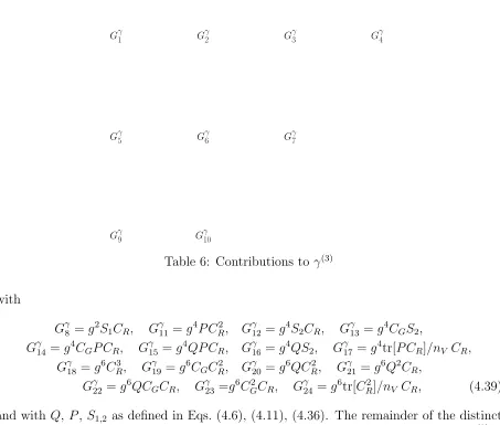
Table 6: Contributions to γ(3)

with

Gγ₈ =g2S1CR, Gγ11=g 4_{P C}2

R, G γ

12 =g 4_S

2CR, Gγ13 =g 4_C

GS2,

Gγ₁₄=g4CGP CR, Gγ15=g 4

QP CR, Gγ16 =g 4

QS2, Gγ17 =g 4

tr[P CR]/nV CR,

Gγ₁₈=g6C_R3, Gγ₁₉ =g6CGCR2, G γ

20 =g6QCR2, G γ

21 =g6Q2CR,

Gγ₂₂=g6QCGCR, Gγ23=g6CG2CR, Gγ24 =g6tr[CR2]/nV CR, (4.39)

and with Q, P, S1,2 as defined in Eqs. (4.6), (4.11), (4.36). The remainder of the distinct tensor contributions are depicted in diagrammatic form in Table (6). The basis for γ(3) _is restricted by the absence of one particle reducible contributions such as P3_{, P}2_C

R, S1,2P,

P S1,2.

Using Eqs. (4.10), (4.25) in Eq. (4.32) leads to a large number of consistency equations which constrainγ(3). If g = 0 they reduce to

2Λ1 =γ1+ Θ3+ 2Θ4 = 2Θ1+ 2Θ2, 2Λ2 = 2γ2+ 2Θ3 = 1 + 2Θ1−Θ˜, 2Λ3 =γ3+ 2Θ4−Θ = 1 + 2Θ˜ 2+ Θ3,

3Λ4 =γ4, (4.40)

which requires

These results were obtained in Ref. [15]. The other special case is forY,Y¯ = 0 when

γ(3) = (γ18−2γ11)g6CR3 + (γ19−2γ14)CG+ (γ20−2γ15)Q

g6C_R2

+ γ21Q2+γ22QCG+γ23CG2 + (γ24−2γ17) tr[CR2]/nV

g6CR. (4.42)

In this case applying Eq. (4.32) with Λ,Θ→0 it is necessary to require the conditions

γ18−2γ11 =−16, γ19−2γ14= 0, (4.43) as well as

γ20−2γ15 = −8−θ˜5+ 2˜θ2, γ21 =−2˜λ3−θ˜3, γ22 =−2˜λ4−θ˜4,

γ23 = −2˜λ5, γ24−2γ17 = 4˜λ1−2˜λ3−4˜θ . (4.44) The relations in Eq. (4.41) were obtained in Refs. [18, 19].

For the general case Eq. (4.32) implies additional relations which further constrain γα.

From terms which start at O((YY¯)2) and using Eq. (4.40)

2Λ5 =γ5+ Θ6+ 4Θ4−2 ˜Θ = 4 + 2Θ5−2 ˜Θ, Λ6 =γ6+ Θ6 = 0, 2Λ7 =γ7 = Θ6,

Λ6+ 4Λ3 =γ8+ 2Θ5−2 ˜Θ,

Λ10= Θ7, Λ11= Θ8, (4.45)

which then entail, using Eq. (4.40) to eliminate Λ3,

γ8+γ5−γ6 = 4 + 2γ3, γ6+γ7 = 0. (4.46) The remaining conditions arise from terms at O(YY¯) which become, using Eq. (4.45) to eliminate Λ5,

2Λ8 =γ9 =γ11−8,

Λ9 =γ10, 2Λ9+ 4Λ7 =γ12, Λ12 =γ16+ 2 ˜Θ + ˜θ1,

Λ12+ 2Λ10 =γ15−4 + 2Θ7+ 2 ˜Θ + ˜θ2,

Λ13 =γ13, Λ13y+ 2Λ11=γ14+ 2Θ8,

−2˜λ1 =γ17−2˜θ , (4.47)

which then give

Altogether Eqs. (4.41), (4.43), (4.46), (4.48) give eight conditions which are all satisfied by the coefficients as calculated [21, 22]:

γ1 =−1, γ2 =−1₂, γ3 = 2, γ4 = 1₄κ, γ5 =−2κ+ 4,

γ6 =−κ, γ7 =κ, γ8 =κ+ 4, γ9 =−5κ, γ10=κ,

γ11=−5κ+ 8, γ12= 4κ, γ13 =−κ, γ14=−κ, γ15=−2,

γ16=−4, γ17 =−12, γ18 =−10κ, γ19=−2κ, γ20=−8,

γ21 = 2, γ22= 4κ+ 12, γ23 = 12κ, γ24=−4κ, (4.49) where κ = 6ζ(3). As mentioned earlier, the NSVZ form of the gauge β-function βg is

valid only in a specific renormalisation scheme (which differs from DRED at three loops). We are therefore obliged for consistency to use the result for the anomalous dimension corresponding to this NSVZ scheme. The required transformation was presented in Ref. [39] and its effect on γ(3) _{given in Ref. [40]. In fact it is only γ}

17 and γ22 which are affected. Once the conditions on the γα in Eqs. (4.41), (4.43), (4.46), (4.48) are satisfied, the

Λα, Θα etc maybe be assigned in accord with Eq. (4.47), with considerable arbitrariness;

there is little to be gained from stating the residual relations amongst them.

In the Wess-Zumino case considered in Ref. [15] the existence of ana-function satisfying Eq. (1.2) implied thatγ1−2γ2−γ3 was an invariant (in a sense described in Ref. [15]) but did not impose a specific value; thus showing that Eq. (4.17) is sufficient but not necessary. We might expect similar remarks to apply to the other conditions in Eq. (1.2). It is all the more striking that these conditions are in fact satisfied by the anomalous dimension as computed.

We may count the independent parameters in the anomalous dimension as we did in Section 2 for the Yukawa β-function. The essential Eqs. (4.13) and (4.17) are invariant under redefinitions of g as in Eq. (4.8) and taking δY =Y ∗h where

δβY =Y ∗δγ , δβ_Y¯ =δγ∗Y ,¯ (4.50) and also assuming δβ˜g is given in terms of δγ in accord Eq. (4.5), for

δγ=− δg∂g+ (Y ∗h)◦∂Y

γ +β_Y¯ ◦∂_¯

Yh . (4.51)

Taking

h= ˜α S1+ ˜β g4S2 + ˜γ g2P CR+ ˜δ g4CR2 + (˜ζ Q+ ˜ξ CG)g4CR,

δg=g5(˜µ Q2+ ˜ν QCG+ ˜ρ CG2 + ˜σtr[C

2

GN P

1 GN P2

Table 7: Non planar Feynman diagrams used to define γ0(3)

results in

δγ1 = 2 ˜α, δγ2 = ˜α, δγ5 = 2 ˜α+ ˜β−˜γ, δγ6 = ˜β,

δγ7 =−β,˜ δγ8 = ˜γ−2 ˜α, δγ9 =−δ,˜ δγ11 =−δ,˜

δγ12=−2 ˜β, δγ13=−ξ,˜ δγ14 =−ξ,˜ δγ15=−ζ,˜

δγ16=−ζ,˜ δγ18=−2˜δ, δγ19 =−2 ˜ξ, δγ20=−2˜ζ,

δγ21 = 4˜µ, δγ22= 4˜ν, δγ23 = 4 ˜ρ, δγ24 = 4˜σ, (4.53) which leave Eqs. (4.41), (4.43), (4.46), (4.48) invariant. Allowing for such variations the number of independent parameters is therefore 24− 10 = 14 but the eight constraints in Eqs. (4.41), (4.43), (4.46), (4.48) reduce the number of free parameters in γ(3) _{to be} reduced to six.

In the g = 0 case, the only coefficient in γ(3) _{with a κ-dependence, γ}

4, corresponds to a non-planar graph. In the general case there is no such obvious association between non-planar Feynman graphs and coefficients in γ(3) with κ-dependence (evaluated using DRED). However, an intriguing observation is that a redefinition given by choosing

˜

β =κ, γ˜=−κ, δ˜=−2κ,

˜

ν =−κ, ρ˜=−3κ, σ˜ =κ , (4.54) (and the remaining coefficients in Eq. (4.52) set to zero) gives a redefined γ(3)

γ0(3) =γ(3)|κ=0+γ4Gγ4+κG NP

1 + 2κG NP

2 , (4.55)

where

GNP₁ =Gγ₉ +Gγ₁₀+g4(−2CRS2+P CR2 +CGS2−CGP CR) + 2g6(CR3 −CGCR2),

GNP₂ =Gγ₉ −Gγ₁₀+g4(P C_R2 +CGP CR) + 2g6(CR3 +CGCR2), (4.56)

5

Reduction of non-supersymmetric results to

super-symmetric case

In this section we shall check that the a-function obtained using the methods of Section 2 for a general theory is compatible, upon specialisation to the supersymmetric case, with the a-function presented in Section 4 (at least up to two loops). The reduction of the non-supersymmetric theory presented in Section 2 to the supersymmetric case (with nψ =

nV +nC, nϕ = 2nC) may be accomplished by writing

ϕa →

φi

¯

φi

, φ¯i = (φi)∗, ψi →

ψi

λA

, i= 1. . . nC, (5.1)

and with yaϕa=yiφi + ¯yiφ¯i,

yi →



  

Yijk _{0 0 0}

0 0 0 0

0 0 0 √2g(RB)ji

0 0 √2g(RT

A)ik 0

    , ¯

yi →



  

0 √2g(RT

B)ji 0 0

√

2g(RA)ik 0 0 0

0 0 Y¯ijk 0

0 0 0 0



  

, (5.2)

where λ is the gaugino field. ˆy¯i and ˆyi may be obtained from ¯yi and yi by interchanging

the upper left and lower right 2×2 blocks of the 4×4 matrices. We also have

tϕ_A→

RA 0

0 −RT A

, tψ_A →

RA 0

0 Rad

A

, (Rad_A)BC =−ifABC, (5.3)

and consequently, from Eq. (2.6),

Rϕ →2TR, Rψ →TR+CG. (5.4)

The scalar potential is now given by

V = 1₄Y¯ijmYklmφ¯iφ¯jφkφl−g2 1₂( ¯φRAφ)( ¯φRAφ). (5.5)

In making the reduction from the general theory to the supersymmetric case, we must start from two-loop β-functions corresponding to DRED, since the RG functions used in Section 3 were evaluated using this scheme; as we mentioned earlier, the DRED and NSVZ schemes coincide up to the two-loop order we are considering in this Section. We use the results given in Ref. [42], which may be obtained from the DREG results by a coupling redefinition as in Eq. (2.17) given by

GS₁ GS₂ GS₃ GS₄

GS₅ GS₆ GS₇ GS₈

Table 8: Contributions to A(4) _{in the supersymmetric case}

with all other coefficients set to zero.4 We list here the values of the coefficients in Eq. (2.16) which change under this redefinition (as may be easily checked using Eqs. (2.19), (2.16)):

cDR₆ = 2 cDR₇ =−1, cDR₁₃ =−5

4, c

DR

14 = 14, c DR 15 = 72,

cDR₁₉ = 7, cDR₂₀ =−1

12 138CG−12R

ψ_−9Rϕ ,

cDR₂₆ = 7₂, cDR₂₈ = ₁₂1(59CG+ 4Rψ +Rϕ), (5.7)

The DREDβ-function leads to the following alterations in the coefficients in Eq. (2.26); the others are the same as in Eq. (2.31).

ADR₁₃ =−5 24, A

DR 14 =−

1 12, A

DR 15 =

7 12, A

DR 16 =−

1 3, A

DR 17 =

1 6,

ADR₁₉ = 1₆, ADR₂₀ = ₄₈5 , ADR₂₂ = 1₄, ADR₂₃ = 1₂, ADR₂₅ =−5 2,

ADR₂₆ =−1

72[138CG−12R

ψ _−9Rϕ_]−t

1β0,

ADR₂₇ = 1

144[59CG+ 4R

ψ_+Rϕ_]−t

2β0, (5.8) These changes are a consequence of making the transformations Eq. (5.6) and also

δg=− g

3

72nV

tr[yayˆaCˆRψ], (5.9)

uponA(3) _{and A}(2) _{respectively in Eq. (2.12). Presumably the transformation in Eq. (5.9)} represents a part of the two-loop transformation from DREG to DRED (namely the Yukawa dependent contribution to the transformation of g). To the best of our knowledge this has

4_{In general the DRED β-functions obtained using (5.6) do not correspond to a diagrammatic}

not been computed in full, though results have been given for the pure gauge case in Ref. [43].

Inserting Eqs. (5.2), (5.3), (5.5) into the expressions for the various contributions to ˜

A(4), depicted in Table (8), we find

GA₁ →2(GS₁ −9GS₃ + 6GS₄ + 6GS₅ −12GS₆ −3(CG−2TR)GS7 + 4GS8 . . .)

GA₂ →6(GS₂ + 2GS₃ −4GS₄ −6GS₅ + (CG−2TR)GS7 +. . .)

GA₃ → −5GS₃ + 16GS₅ −16GS₆ + 4CGGS7 + 2G

S

8 +. . .

GA₄ →2(9GS₅ −6GS₆ + 3CGGS7 +G

S

8 +. . .), G

A

5 →2(G

S

1 −6G

S

3 + 12G

S

5 +. . .)

GA₆ →2(GS₂ −4GS₄ + 4GS₆ −8TRGS7 +. . .),

GA₇ →2S2−4GS3 −12G

S

4 + 24G

S

5 + 16G

S

6 −8TRGS7 +. . . ,

GA₈ →2GS₁ −24GS₃ + 96GS₅ +. . .

GA₉ →2(GS₃ + 2GS₄ −2GS₅ −4GS₆ + 2TRGS7 +. . . G

A

10 →2(−G

S

3 + 4G

S

5 +. . .)

GA₁₁→4(2GS₃ −8GS₅ +. . .), GA₁₂→4(GS₄ + 2GS₅ +. . .)

GA₁₃→2(GS₃ −4GS₅ +. . .), G₁₄A →2(GS₄ −2G₆S+ 2CGGS7 +. . .)

GA₁₅→2(GS₄ −2GS₅ −2GS₆ +. . .) GA₁₆→2(GS₅ + 2GS₆ −CGGS7 +. . .), G

A

17 →8G

S

5 +. . .

GA₁₈→ 1 2G

S

3 −4G

S

5 −2CGGS7 +. . . , G

A

19 →2G

S

4 −4G

S

5 −8G

S

6 + 4CGGS7 +. . . ,

GA₂₀→2GS₃ −16GS₅ . . . , GA₂₁ →3GS₅ −2GS₆ + ₂1CGGS7 +. . . , G

A

22 →2G

S

5 +. . .

GA₂₃→2GS₆ +. . . , GA₂₄ →4GS₅ +. . . , GA₂₅ →4GS₆ +. . . GA₂₆→2GS₇ +. . . , GA₂₇ →2GS₇ +. . . ,

GA₂₈→ 3 2G

S

1 + 3G

S

2 + 12G

S

3 + 24G

S

4 + 24G

S

5 + 48G

S

6 +. . . , (5.10)

where again we do not display the purely gauge-coupling dependent terms.

It is then straightforward to show, using the DRED values of the coefficients from Eqs. (2.31), (5.8) that ˜A(4) _{reduces as}

˜

A(4) → 1 3tr[(γ

(1)

)3] + α− 1 36

β_Y(1)◦β(1)_¯

Y +

−1

2 + 8(t1+t2)

β_g(1)gtr[P CR]. (5.11)

This expression can readily be shown, with the aid of Eqs. (4.10), (4.5), to be equivalent at this order to Eq. (4.13). The explicit form at this order was already given in Ref. [20]; with our notation and conventions, this corresponds to Λ(1) _{=Y as in Eq. (4.22) and with}

βY ◦H◦β_Y¯ =α β_Y ◦β_Y¯ , (5.12)

and

λ=g2+ ˜λg4Q+ ˜

λ1

nV

g4tr[P CR] +. . . , (5.13)

where we have picked out the terms which can contribute to Qtr[P CR]. We find using

Eqs. (4.5), (4.31), (4.47), (4.49), (5.11) that we require

t1+t2 = 29

These coefficients correspond to a three-loop calculation (see Eq. (2.23)) and, in view of Eq. (4.47), depend on the value of γ17, which has a different value for the NSVZ scheme than for DRED. It is beyond the scope of this article to consider how Eq. (5.14) would be modified within DRED or indeed within DREG. Since our whole approach is predicated on the NSVZ scheme, it would probably be naive to assume that the DRED form of Eq. (5.14) would be obtained simply by using the DRED result for γ17.

Eq. (5.11) extends the result of Eq. (7.30) in Ref. [15] (with a= 3α− 1

12) to the gauge case–once again, modulo pure gauge terms which are not captured by the methods used in Section 2. We see again the ambiguity in the form of ˜A expressed in general by Eq. (2.27). Of course this check is guaranteed to work but nevertheless given the indirect manner in which we have obtained ˜Aand the possibility of subtleties regarding scheme dependence, it is satisfying to “close the loop” in this fashion.

Finally, we remark that although the form for ˜A presented in Eq. (5.11) is appealingly simple (arguably even more so than Eq. (4.13)), the obvious extension to higher loops does not appear to be viable.

6

Conclusions

In this article we have extended the results of Ref. [15] to the case of general gauge theories. In the non-supersymmetric case we have constructed the terms in the four-loop a-function containing Yukawa or scalar contributions, using the two-loop Yukawaβ-function and one-loop scalar β-function. Our main result here is Eq. (2.26) with Eq. (2.31). This enabled a comparison with similar terms in the three-loop gauge β-function. In general, as a consequence of the properties of the coupling-constant metric, one can obtain information on the (n+ 1)-loop gaugeβ-function from then- (and lower-) loop Yukawaβ-function and the (n−1) (and lower) loop scalarβ-function. This is reminiscent of the way in which the (n+ 1)-loop gauge β-function is determined by the lower order anomalous dimensions in a supersymmetric theory, via the NSVZ formula.

In the supersymmetric case we have given a general sufficient condition for the exact

a-function of Refs. [17–19], given in Eq. (4.13), to be valid, and shown that it is satisfied by the three-loop anomalous dimension. This condition is displayed in Eq. (4.17) and is our main result for the supersymmetric case.

One feature of interest is that Eq. (4.17) imposes extra conditions on the anomalous dimension beyond the mere requirements of integrability from Eq. (1.2); but which are nevertheless satisfied by the explicit results as computed. Indeed we remark here (without giving further details since it is beyond our remit in this article on the gauged case) that we have observed similar features in the Wess-Zumino model at four loops, using the results of Ref. [41].

must be satisfied; it would be interesting to explore this further. If this were indeed the case, one could imagine exploiting Eq. (4.17) to expedite higher-order calculations of the anomalous dimension such as the full gauged case at four loops; possibly combined with ad-ditional information such as the necessary vanishing ofγ in theN = 2 case. Unfortunately, a preliminary check indicates that these constraints are far from sufficient to determine γ

completely, even at three loops; and therefore a considerable quantity of perturbative cal-culation would still be unavoidable.

Finally, in Ref. [15] we explored in some detail the freedoms to redefine the various quantities we have considered, and it would be interesting to extend these discussions to the current gauged case. In particular it would be useful to extend Eq. (4.17), which in its current form is predicated upon the NSVZ renormalisation scheme, to a form valid for

any scheme.

7

Acknowledgements

We are very grateful to Tim Jones and Hugh Osborn for useful conversations and for a careful reading of the manuscript. CP thanks the STFC for financial support.

References

[1] J.L. Cardy, Is There a c-theorem in Four Dimensions?, Phys. Lett. B215 (1988) 749. [2] A.B. Zamolodchikov, Irreversibility of the Flux of the Renormalization Group in a 2D

Field Theory, JETP Lett. 43 (1986) 730.

[3] Z. Komargodski and A. Schwimmer, On Renormalization Group Flows in Four Dimen-sions, JHEP 1112 (2011) 099, arXiv:1107.3987 [hep-th]; Z. Komargodski, The Con-straints of Conformal Symmetry on RG Flows, JHEP 1207 (2012) 069, arXiv:1112.4538 [hep-th].

[4] M.A. Luty, J. Polchinski and R. Rattazzi, The a-theorem and the Asymptotics of 4D Quantum Field Theory, JHEP 1301 (2013) 152, arXiv:1204.5221 [hep-th].

[5] H. Elvang, D.Z. Freedman, L.Y. Hung, M. Kiermaier, R.C. Myers and S. Theisen, On renormalization group flows and the a-theorem in 6d, JHEP 1210 (2012) 011, arXiv:1205.3994 [hep-th];

H. Elvang and T.M. Olson, RG flows in d dimensions, the dilaton effective action, and the a-theorem, JHEP 1303 (2013) 034, arXiv:1209.3424 [hep-th].

[7] H. Osborn, Weyl consistency conditions and a local renormalization group equation for general renormalizable field theories, Nucl. Phys. B363 (1991) 486.

[8] B. Grinstein, A. Stergiou and D. Stone, Consequences of Weyl Consistency Conditions, JHEP 1311 (2013) 195, arXiv:1308.1096 [hep-th].

[9] Y. Nakayama, Consistency of local renormalization group in d = 3, Nucl. Phys. B879 (2014) 37, arXiv:1307.8048 [hep-th].

[10] B. Grinstein, A. Stergiou, D. Stone and M. Zhong, A challenge to the a-theorem in six dimensions, arXiv:1406.3626 [hep-th].

[11] J. -F. Fortin, B. Grinstein and A. Stergiou, Scale without Conformal Invariance at Three Loops, JHEP 1208 (2012) 085, arXiv:1202.4757 [hep-th].

[12] J. -F. Fortin, B. Grinstein and A. Stergiou, Limit Cycles and Conformal Invariance, JHEP 1301 (2013) 184, arXiv:1208.3674 [hep-th].

[13] J. -F. Fortin, B. Grinstein, C.W. Murphy and A. Stergiou, On Limit Cycles in Super-symmetric Theories, Phys. Lett. B719 (2013) 170, arXiv:1210.2718 [hep-th].

[14] Yu Nakayama, Supercurrent, Supervirial and Superimprovement, Phys. Rev. D87 (2013) 085005, arXiv:1208.4726 [hep-th].

[15] I. Jack and H. Osborn, Constraints on RG flow for Four-dimensional Quantum Field Theories, Nucl. Phys. B883 (2014) 425.

[16] F. Baume, B. Keren-Zur, R. Rattazzi and L. Vitale, The local Callan-Symanzik equa-tion: structure and applications, arXiv:1401.5983 [hep-th].

[17] D. Anselmi, D.Z. Freedman, M.T. Grisaru and A.A. Johansen, Nonperturbative for-mulas for central functions of supersymmetric gauge theories, Nucl. Phys. B526 (1998) 543, hep-th/9708042;

D. Anselmi, J. Erlich, D.Z. Freedman and A.A. Johansen, Positivity constraints on anomalies in supersymmetric gauge theories, Phys. Rev. D57 (1998) 7570, hep-th/9711035.

[18] E. Barnes, K.A. Intriligator, B. Wecht and J. Wright, Evidence for the strongest version of the 4d a-theorem, via a-maximization along RG flows, Nucl. Phys. B702 (2004) 131, hep-th/0408156.

[19] D. Kutasov, New results on the ‘a-theorem’ in four-dimensional supersymmetric field theory, hep-th/0312098;

[20] D.Z. Freedman and H. Osborn, Constructing a c-function for SUSY gauge theories, Phys. Lett. B432 (1998) 353, hep-th/980410.

[21] A.J. Parkes and P.C. West, Three Loop Results in Two Loop Finite Supersymmetric Gauge Theories, Nucl. Phys. B256 (1985) 340.

[22] I. Jack, D.R.T. Jones and C.G. North, N=1 supersymmetry and the three loop anoma-lous dimension for the chiral superfield, Nucl. Phys. B473 (1996) 308, hep-ph/9603386. [23] O. Antipin, M. Gillioz, E. Mølgaard and F. Sannino, Thea-theorem for Gauge-Yukawa theories beyond Banks-Zaks, Phys. Rev. D87 (2013) 125017, arXiv:1303.1525 [hep-th]. [24] D.J. Wallace and R.K.P. Zia, Gradient Properties of the Renormalization Group

Equa-tions in Multicomponent Systems, Annals Phys. 92 (1975) 142.

[25] J.A. Gracey, D.R.T. Jones and A.G.M. Pickering, Three loop gauge β-function for the most general single gauge coupling theory, Phys. Lett. B510 (2001) 347, hep-ph/0104247.

[26] M.E. Machacek and M.T. Vaughn, Two Loop Renormalization Group Equations in a General Quantum Field Theory. 1. Wave Function Renormalization, Nucl. Phys. B222 (1983) 83; 2. Yukawa couplings Nucl. Phys. B236 (1986) 221; 3. Scalar quartic couplings, Nucl. Phys. B249 (1985) 70.

[27] I. Jack and H. Osborn, General Background Field Calculations With Fermion Fields, Nucl. Phys. B249 (1985) 472.

[28] B. Keren-Zur, The local RG equation and chiral anomalies, arXiv:1406.0869[hep-th]. [29] D.R.T. Jones, More on the Axial Anomaly in Supersymmetric Yang-Mills Theory,

Phys. Lett. B123 (1983) 45.

[30] K.G. Chetyrkin and M.F. Zoller, Three-loopβ-functions for top-Yukawa and the Higgs self-interaction in the Standard Model, JHEP 1206 (2012) 033, arXiv:1205.2892 [hep-ph].

[31] O. Antipin, M. Gillioz, J. Krog, E. Mølgaard and F. Sannino, Standard Model Vacuum Stability and Weyl Consistency Conditions, JHEP 1308 (2017) 034, arXiv:1306.3234 [hep-ph].

[32] V. Novikov et al, Exact Gell-Mann-Low Function of Supersymmetric Yang-Mills The-ories from Instanton Calculus, Nucl. Phys. B229 (1983) 381;

V. Novikov et al, Beta Function in Supersymmetric Gauge Theories: Instantons Versus Traditional Approach, Phys. Lett. B166 (1986) 329;

[33] A. Vainstein, V. Zakharov and M. Shifman, Susy Nonabelian Gauge Models: Exact

β-function From One Loop Of Perturbation Theory, Sov. J. Nucl. Phys. 43 (1986) 1028; M. Shifman, A. Vainstein and V. Zakharov, Exact Gell-Mann-Low Function In Super-symmetric Electrodynamics, Phys. Lett. B166 (1986) 334.

[34] D.R.T. Jones, Asymptotic Behavior of Supersymmetric Yang-Mills Theories in the Two Loop Approximation, Nucl. Phys. B87 (1975) 127.

[35] A.J. Parkes and P.C. West, Finiteness in Rigid Supersymmetric Theories, Phys. Lett. B138 (1984) 99.

[36] D.R.T. Jones and L. Mezincescu, Theβ Function in Supersymmetric Yang-Mills The-ory, Phys. Lett. B136 (1984) 242;

[37] D.R.T. Jones and L. Mezincescu, The Chiral Anomaly and a Class of Two Loop Finite Supersymmetric Gauge Theories, Phys. Lett. B138 (1984) 293.

[38] P. West, The Yukawaβ Function in N=1 Rigid Supersymmetric Theories, Phys. Lett. B137 (1984) 371.

[39] I. Jack, D.R.T. Jones and C.G. North, N = 1 supersymmetry and the three loop gauge β function, Phys. Lett. B386 (1996) 138, hep-ph/9606323.

[40] I. Jack, D.R.T. Jones and C.G. North, Scheme dependence and the NSVZ β function, Nucl. Phys. B486 (1997) 479, hep-ph/9609325.

[41] P.M. Ferreira, I. Jack and D.R.T. Jones, The quasi-infra-red fixed point at higher loops, Phys. Lett. B392 (1997) 376, hep-ph/9610296.

[42] I. Jack, Two Loop Beta Functions for Supersymmetric Gauge Theories, Phys. Lett. B147 (1984) 405.

[43] L. Mihaila, Two-loop parameter relations between dimensional regularisation and di-mensional reduction applied to SUSY-QCD, Phys. Lett. B681 (2009) 52.

[44] R. van Damme and G. ’t Hooft, Breakdown of Unitarity in the Dimensional Reduction Scheme, Phys. Lett. B150 (1985) 133.