A Statistical Analysis Of Migration Using Logistic Regression Model

(1)

1331

A Statistical Analysis Of Migration Using Logistic

Regression Model

Dr. G. Venkatesan, V. Sasikala ,

Abstract : In this paper, statistical analysis is carried out using logistic regression model and the study shows the significant status between Tamilnadu and India with reference to different indicators. Migration in India and as well as Tamilnadu influenced by its pattern of economic development. In particular, this study is to analyse male migrants’ duration of stay as a risk factor for migration according to various reasons and to analyse the distribution pattern of male migrants regarding economic activity for employment in Tamilnadu and India using secondary data from census of India during the census years 2001 and 2011.

Key words: Census years, logistic regression, migration, odds ratio, Wald’s statistic .

——————————  ——————————

1 INTRODUCTION

Logistic Regression has been used in the biological sciences in early twentieth century. It was then used in many social science applications. A logistic regression model allows us to establish a relationship between a binary outcome variable and a group of predictor variables. It models the logit-transformed probability as a linear relationship with the predictor variables. Zezula (2010), explained the various types of regression by giving examples using software. Nurullah and Rafiqul Islam (2011) studied the determinant of socio- demographic characteristics on female migrants using logistic regression model and concluded that most of the female migrants are migrated to urban areas due to marriage for better life. John G.Eastwood and et al., (2013) studied to explore the multilevel spatial distribution of depressive symptoms among migrant mothers in South Western Sydney. By using Bayesian hierarchical multilevel spatial modelling, it is found that multicultural home visiting support is required for migrant mothers living in more communities where they may have poor social networks. Guoqi Li and et al., (2015) studied an entropy-based method is proposed to three stage forecast demographical changes of counties and estimated the demographic trends by using entropy as an optimization variable. Jorge Garza-Rodriguez, Jennifer Fernandez-Ramos and Ana K. Garcia-Guerra, Gabriela Morales-Ramirez(2015) studied the dynamics of poverty in Mexico using multinomial logistic regression analysis based on transition matrices of households and shows that gender of the household head differentiates chronically poor and transiently poor whereas age of the household head differentiates the probability of escaping poverty. Pandey A.P (2016), studied the motivation to farmers to engage in contract farming mechanism related to socio-economic factors by using logistic regression approach which reveals that small hold farmers are even eager to adopt contract farming mechanism.

O Singh and Urbashi Pandey (2017) studied a logistic analysis between internal migration in Almora district of

Uttarakhand to identify the socio-economic and

demographic factors affecting on migration by taking 750 respondents and concludes that employment is main cause of migration for males and lack of basic needs have no motivation to return migration to that district. Jung In Seo and Yongku Kim (2017) have studied an entropy inference method based on an objective Bayesian approach for two parameter Logistic distribution using non-informative priors through the posterior predictive checking based on the replications of the observed upper record values. James Flamino and et al., (2017) explained a predictive algorithm for the smart growth of cities with populations and it estimated the growth of a city from smart growth proposal assessed by a logistic weight model. Christiane Von Reichert and Gundars Rudzitis studied multinomial logistic models explain income changes of migrants to identify the impact of migrant’s characteristics and their satisfaction level of pull and push factors on income change and concluded that higher age migrants were more inclined to accept lower income than younger migrants. Our aim is to study the problem of migrants’ stay duration dependent with gender according to various reasons and compare the effectiveness of migration between employment status for economic development in India and Tamilnadu between census years 2001 and 2011. In this study multiple logistic regression and multinomial logistic regression model approaches has been used to construct the statistical analysis.

2 MATERIALS AND METHODS

2.1 Generalized linear model

In generalized linear model, a random variable Y from a distribution is considered as a function of a dependent variable X. The linear part becomes a function g(.) (say) of

the mean , - is modelled as a linear function XT β.

That is * , -+ = XT β. Here g(.) is called the link

function and is dependent on the distribution yi , for all i = 1,2,..m, m being dimension of Y.

2.2 Multiple Logistic Regression

Logistic Regression is used to predict the dependent variable which is categorical on the basis of independent variables. It has many types. The former type is Binary Logistic Regression where the categorical response has

_______________________

Dr. G. Venkatesan, Associate Professor and Head (Rtd.), Department of Statistics, Government Arts College (Autonomous), Salem-636007, Tamilnadu, India, Ph: 9442211562, E-mail:venkatesang1959@gmail.com

(2)

1332

only two possible outcomes. Example: Whether place of birth of a respondent is rural? the answer may be yes or no, secondly, Multinomial Logistic Regression which has three or more categories without ordering. Example: Predicting which age group is preferred more (0-10, 10-20, 20+) and the third type be Ordinal Logistic Regression which has three or more categories with ordering. Example: satisfaction level rating from 1 to 5. In logistic regression the log odds are modelled as a linear function of independent

variables. Multiple logistic regression is used when there

are more than one independent variables under study. The

assumption of logistic regression is, binary logistic

regression requires the dependent variable to be binary, secondly logistic regression requires the observations are to be independent of each other, thirdly the independent variables should not be too highly correlated with each other and assumes linearity of independent variables and log odds, and lastly logistic regression typically requires a large sample size. For example, if you were studying the presence or absence of an infectious disease and had subjects who were in close contact, the observations might not be independent; if one person had the disease, people near them (who might be similar in occupation, socioeconomic status, age, etc.) would be likely to have the disease.

Let ⁄ ( ) then, [ ⁄ ]

./ ∑ (1)

which gives m+1 parameter and it is known as standard

linear model for any explanatory variables . To

solve this equation for , the exponential function is applied

for both sides of equation (1),

{ ./} ( ∑ ) (2) ./ ( ∑ ) (3) multiply both sides by 1-pi , equation (3) becomes,

( ) ( ∑

)

( ∑ ) ( ∑ )

+ ( ∑ ) ( ∑ )

( ( ∑ )) ( ∑ ) (4)

* ∑ +

* ∑ + and

* ∑ + (5)

which implies

* | + ∑

∑ and

* | +

∑ (6)

is known as the logistic model of Y with respect to X. The parameters can be estimated by using maximum likelihood principle in the form of log odds ratio.

2.3 Multinomial Logistic Regression

Logistic regression is an extension of logit models if one or more of the independent variables are quantitative. It can be used with a binomially or multinomially distributed dependent variable. It coincides simple linear logistic model on the case of dichotomic outcome. Multinomial logistic regression compares multiple groups through a combination of binary logistic regression. The group comparisons are equivalent the comparison between dependent variable with the highest numeric score group used as the reference group. The multinomial model allows

each category of dependent variable to be comparted with reference category providing a number of logistic

regression models. For example People’s occupational

choices might be influenced by their parents’ occupations and their own education level. We can study the relationship of one’s occupation choice with education level and father’s occupation. The occupational choices will be the outcome variable which consists of categories of

occupations. The jth multinomial logistic regression model

is given by, .

/ (7)

2.4 Odds Ratio

Odds ratio is associated with regression coefficient. Because, odds ratio is a measure of the risk for the predictors. Consider ratio of Y=1 Vs Y=0 for a given set of

attributes and also odds can be written as,

* | + * | +

∑ ∑

∑

∑ ₍₈₎

if is incremented by one unit, equation (2.4.1) becomes,

( ) ( ) ∑ ₍₉₎

Hence, odds ratio is given by,

( ₍ ₎) ( ) ∑_{( ) ∑}

*( ( ) ∑ )

( ( ) ∑ )+

(10)

also, by taking natural logarithm on both sides in the above equation,

{ ( )

( )} ̂ (11)

and ̂ be the Y intercept which is log of odds be the

estimated parameters.

2.5 Testing of goodness of fit

Under H0, significance tests can be performed for regression coefficients by using Wald statistic which has asymptotically normal with mean 0 and variance 1 and its square is approximately follows chi-square with one degrees of freedom. The significance can be interpreted by p value.

2.6 Wald’s test

The Wald test (also called the Wald Chi-Squared Test) is used whether the explanatory variables in a model are significant or not. If the Wald test shows that the parameters for certain explanatory variables are zero, we remove the variables from the model otherwise we include the variables in the model. The Wald test is usually termed as an alternative form of chi-squared because sample size approaches infinity, and hence the test is sometimes called the Wald Chi-Squared Test. Wald

statistic is used for testing the hypothesis that

against the alternative . The Wald statistic is

calculated using the formula ₍̂_̂₎ ( ). The

distribution of the Wald statistic is closely approximated by the normal distribution in large samples. However, in small samples, the normal approximation may be poor.

(3)

1333

2.7 Reference Value

When using multinomial logistic regression, one category among m categories of the dependent variable is chosen as the reference category. The reference value is that category of the Y variable that is defined implicitly in terms of the other categories. One explanatory variable is replaced by m-1 indicator variables of other categories, which are mutually exclusive. Regression coefficient indicates significant difference between corresponding category and the reference category.

3 MIGRATION MODELS

3.1 Multiple Logistic Regression for migration

Consider a random variable Y (Dependent variable) which is dichotomic.

ie., Y = 1 if migrant is male

0 otherwise (migrant is female)

and X be independent categorical variable which is grouped in to 4 categories as a risk factor for male migrants.

1 if duration of stay is <1 year

ie., X = 2 if duration of stay is 1-4 years

3 if duration of stay is 5-9 years 4 if duration of stay is >10 years

The Logistic model for migration using equation (1) is given by,

./ (12)

where pi is the probability of an event that male migrant’s

duration of stay under ith category; i = 1,2,3,4. The

observed values are shown in contingency table. The solution for the corresponding parameters are done through MLE.

That is, ̂

and ̂

, (13)

i = 1,2,…m and j = 1,2,…n.

Also,

̂ ̂ ̂ _̂

and , (14)

where nij (i=1,2,3,4 ; j=1,2) be the observed values and m be the number of predictor categories or independent variable

categories and hence ̂ ( ) . /, i = 1,2,3

(15)

are the estimated parameter values where one category is taken as reference.

3.2 Multinomial Logistic Regression for migration:

Consider two multinomial distributions with probabilities pij ;

i = 1, 2,…,m; j = 1,2,…,n of migrants economic activity for employment during census years 2001 and 2011 in Tamilnadu and India respectively. Since one of the probabilities in each row is redundant, let us choose one response category as a reference.

Let (

) (16)

be the multinomial logistic regression model.

1 if migrant belongs to main workers

Let Y = 2 if migrant belongs to marginal workers

3 if migrant belongs to non-workers be a dependent variable and X be independent variable which is grouped in to 2 categories namely male and

female. That is xi ɛ {0,1} is the indicator of gender. In our

problem non-workers category is chosen as reference to

describe the behaviour of Y which indicates male migrants. Hence, the multinomial logistic model for migration is given by,

.

/ (17)

where pij is the probability of an event that migrant’s

economic activity for employment. The parameters be

the differences of log-odds for jth response category (j=1,2)

to the reference category. Taking the logarithm of the ratio turns to be difference of the log-likelihoods.

3.3 Source of data

The secondary data is collected from, Census of India (D-Series migration tables) during census years 2001 and 2011 for Tamilnadu and India.

4 STATISTICAL ANALYSIS AND RESULT

DISCUSSIONS

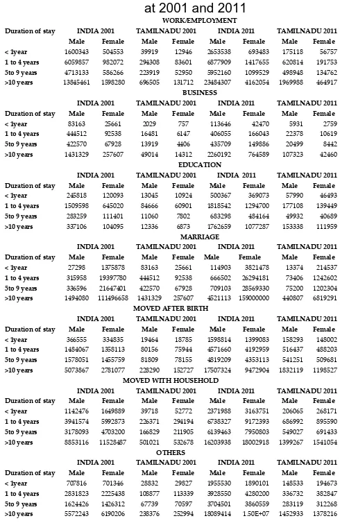
Table 1

Distribution of migrants with gender and duration of stay according to reasons in India and Tamilnadu

at 2001 and 2011

Table 1 shows the distribution of migrants by sex and

duration of residence according to reasons

(Work/Employment, Business, Education, Marriage, moved after birth, moved with household and others) in Tamilnadu and India for the census years 2001 and 2011.

To test the null hypothesis (H0) that Duration of stay of male migrants as a risk factor for migration according to reasons

Duration of stay

WORK/EMPLOYMENT

INDIA 2001 TAMILNADU 2001 INDIA 2011 TAMILNADU 2011 Male Female Male Female Male Female Male Female < 1year 1600343 504553 39919 12946 2653538 693483 175118 56757

1 to 4 years 6059857 982072 294308 83601 6877909 1417655 620814 191753

5to 9 years 4713133 586266 223919 52950 5952160 1099529 498948 134762

>10 years 13845461 1598280 696505 131712 23484307 4162054 1969988 464917

BUSINESS

INDIA 2001 TAMILNADU 2001 INDIA 2011 TAMILNADU 2011 Duration of stay Male Female Male Female Male Female Male Female < 1year 83163 25661 2029 757 113646 42470 5931 2759

1 to 4 years 444512 92538 16481 6147 406055 166043 22378 10619

5to 9 years 422570 67928 13919 4406 435709 149886 20499 8442

>10 years 1431329 257607 49014 14312 2260192 764589 107323 42460 EDUCATION

1 to 4 years 1509598 645020 84666 60901 1818542 1294700 177108 139449

5to 9 years 283259 111401 11060 7802 683298 484164 49932 40689

>10 years 337106 104095 12336 6873 1762659 1077287 153338 111959

MARRIAGE

1 to 4 years 315958 19397780 444512 92538 666502 26294181 73406 1242602

5to 9 years 336596 21647401 422570 67928 709103 28569330 75200 1202304

>10 years 1494080 111496658 1431329 257607 4521113 159000000 440807 6819291

MOVED AFTER BIRTH

1 to 4 years 1484067 1358113 80156 75944 4571660 4192959 516437 488203

5to 9 years 1578051 1455759 81809 78155 4819209 4353113 541251 509681

>10 years 5073867 2781077 228290 152727 17507324 9472904 1832119 1198527

MOVED WITH HOUSEHOLD

1 to 4 years 3941574 5992873 226371 294194 6738327 9172393 686992 895590

5to 9 years 3178093 4703200 166829 211905 6139463 7950803 549027 691433

>10 years 8853116 11528487 501021 532678 16203938 18002918 1399267 1541054

OTHERS

1 to 4 years 2831823 2225438 108877 113339 3928550 4280200 336732 382847

5to 9 years 1624426 1426312 67739 70597 3704501 3860559 283119 312268

(4)

1334

(Work/Employment, Business, Education, Marriage, moved after birth, moved with household and others) in Tamilnadu and India during census years 2001and 2011, multiple logistic regression model described in equation (12) is applied with the above data, the results obtained and presented in table 2 and table 3.

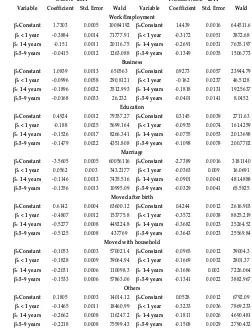
Table 2

Estimated Beta coefficients using multiple logistic regression model for India and Tamilnadu in 2001

Table 2 shows that estimated values of parameters using multiple logistic regression model have lesser p value (<0.05) of Wald Statistic which indicates that duration of stay for male migrants as a risk factor which influence the migration with highly significant according to reasons (work/employment, education, marriage etc.,) for both Tamilnadu and India during census year 2001.

Table 3

Estimated Beta coefficients using multiple logistic models for India and Tamilnadu in 2011

Table 3 shows that estimated values of parameters using multiple logistic regression model have lesser p value (<0.05) of Wald Statistic which indicates that duration of stay for male migrants as a risk factor which influence the migration with highly significant according to reasons (work/employment, education, marriage etc.,) for both Tamilnadu and India during census year 2011.

Table 4 shows the distribution of migrant’s economic

activity under employment for India and Tamilnadu in 2001.

Table 4

Contingency table for migrants' distribution regarding economic activity for India and Tamilnadu in 2001

Table 5

INDIA - 2001 TAMILNADU - 2001 Variable Coefficient Std. Error Wald Variable Coefficient Std. Error Wald

Work/Employment

β0 Constant 2.159 0.0008 6225047 β0 Constant 1.6655 0.003 230301.9

β1 < 1 year -1.0047 0.0018 305466.5 β1 < 1 year -0.5394 0.0106 2613.513

β2 1-4 years -0.3393 0.0014 61181.09 β2 1-4 years -0.4069 0.0049 6788.581

β3 5-9 years -0.0747 0.0016 2132.947 β3 5-9 years -0.2235 0.0057 1542.992

Business

β0 Constant 1.7149 0.0021 729444.1 β0 Constant 1.231 0.0095 14657.21

β1 < 1 year -0.5391 0.0075 5229.381 β1 < 1 year -0.2451 0.0436 31.5422 β2 1-4 years -0.1456 0.0042 1201.448 β2 1-4 years -0.2448 0.0177 191.0183

β3 5-9 years 0.113 0.0047 589.1151 β3 5-9 years -0.0807 0.0197 16.7465

Education

β1 < 1 year -0.4588 0.005 8429.543 β1 < 1 year -0.4075 0.0199 420.6069

β2 1-4 years -0.3248 0.0038 7133.839 β2 1-4 years -0.2555 0.016 256.1233

β3 5-9 years -0.2419 0.005 2332.547 β3 5-9 years -0.236 0.0211 125.082 Marriage

β0 Constant -4.3125 0.0008 25560166 β0 Constant -3.3364 0.0032 952095.1 β1 < 1 year 0.3925 0.0062 4049.052 β1 < 1 year 0.2492 0.0225 122.3626

β2 1-4 years 0.1952 0.002 9780.969 β2 1-4 years 0.2069 0.0073 810.8627

β3 5-9 years 0.1487 0.0019 5985.733 β3 5-9 years 0.1993 0.0072 773.9274

Moved after birth

β1 < 1 year -0.5108 0.0025 41597.36 β1 < 1 year -0.3665 0.0107 1162.298

β2 1-4 years -0.5126 0.0014 133584 β2 1-4 years -0.348 0.006 3311.188

β3 5-9 years -0.5206 0.0014 144371.7 β3 5-9 years -0.3563 0.006 3531.044

Moved with household

β0 Constant -0.2641 0.0004 769338.8 β0 Constant -0.0613 0.002 14768.47

β1 < 1 year -0.1035 0.0013 6367.105 β1 < 1 year -0.2229 0.0069 1035.155

β2 1-4 years -0.1549 0.0008 38702.94 β2 1-4 years -0.2008 0.0034 3449.024

β3 5-9 years -0.1279 0.0009 22505.72 β3 5-9 years -0.1779 0.0038 2169.698 Others

β0 Constant -0.1052 0.0006 49606.79 β0 Constant -0.0595 0.0029 209.605 β1 < 1 year 0.1144 0.0018 4112.654 β1 < 1 year 0.0256 0.0087 8.5749

β2 1-4 years 0.3461 0.0011 104777.2 β2 1-4 years 0.0194 0.0051 14.3182

β3 5-9 years 0.2352 0.0013 33380.01 β3 5-9 years 0.0182 0.0061 8.9254

INDIA - 2011 TAMILNADU - 2011 Variable Coefficient Std. Error Wald Variable Coefficient Std. Error Wald

Work/Employment

β0 Constant 1.7303 0.0005 10084192 β0 Constant 1.4439 0.0016 644511.6 β1 < 1 year -0.3884 0.0014 71777.91 β1 < 1 year -0.3172 0.0051 3872.68 β2 1-4 years -0.151 0.0011 20116.75 β2 1-4 years -0.2691 0.0031 7635.197 β3 5-9 years -0.0415 0.0012 1263.088 β3 5-9 years -0.1349 0.0035 1506.773

Business

β0 Constant 1.0839 0.0013 650563 β0 Constant 0.9273 0.0057 23944.79 β1 < 1 year -0.0996 0.0058 290.8121 β1 < 1 year -0.162 0.0237 46.5128 β2 1-4 years -0.1896 0.0032 3512.993 β2 1-4 years -0.1818 0.0131 192.5637 β3 5-9 years -0.0168 0.0033 26.232 β3 5-9 years -0.0401 0.0141 8.0452

Education

β0 Constant 0.4924 0.0012 79357.27 β0 Constant 0.3145 0.0039 2711.63 β1 < 1 year -0.188 0.0025 5699.164 β1 < 1 year -0.0935 0.0074 161.4259 β2 1-4 years -0.1526 0.0017 8266.341 β2 1-4 years -0.0755 0.0053 201.3698 β3 5-9 years -0.1479 0.0022 4351.808 β3 5-9 years -0.1098 0.0078 200.7702

Marriage

β0 Constant -3.5605 0.0005 60056116 β0 Constant -2.7389 0.0016 3181140 β1 < 1 year 0.0562 0.003 343.2177 β1 < 1 year -0.0363 0.009 16.0691 β2 1-4 years -0.1146 0.0013 7435.516 β2 1-4 years -0.0901 0.0041 481.4888 β3 5-9 years -0.1356 0.0013 10995.09 β3 5-9 years -0.0329 0.0041 65.5825

Moved after birth

β0 Constant 0.6142 0.0004 63600.12 β0 Constant 0.4244 0.0012 2616.903 β1 < 1 year -0.4807 0.0012 153775.8 β1 < 1 year -0.3572 0.0038 8825.219 β2 1-4 years -0.5277 0.0008 449224.8 β2 1-4 years -0.3682 0.0023 25264.52 β3 5-9 years -0.5125 0.0008 437769 β3 5-9 years -0.3643 0.0023 25569.84

Moved with household

β0 Constant -0.1053 0.0003 570021.4 β0 Constant -0.0965 0.0012 39004.3 β1 < 1 year -0.1828 0.0009 39064.94 β1 < 1 year -0.1669 0.0032 2801.37 β2 1-4 years -0.2031 0.0006 110098.3 β2 1-4 years -0.1686 0.002 7226.064 β3 5-9 years -0.1533 0.0006 57863.06 β3 5-9 years -0.1341 0.0022 3882.967

Others

(5)

1335

Odds and Log odds for India and Tamilnadu by taking

reference category as non-workers - 2001

From table 5 and by using equation (17), for census year 2001, the two multinomial logistic regression models for main workers and marginal workers categories are obtained as Y = -1.054 + 1.464 X0 and Y = -1.308 - 0.614 X0

respectively. That is, ( )

( ) be the log odds and

( ) and ( )

be the difference between of log odds for India.

Similarly, the two multinomial logistic regression models for Tamilnadu using equation (17) are Y = -0.754 +1.235 X0 and Y = -1.880 + 0.079 X0 respectively.

Table 6 shows the distribution of migrant’s economic activity under employment for India and Tamilnadu in 2011.

Table 6

Contingency table for migrants' distribution regarding economic activity

for India and Tamilnadu in 2011

Table 7

Odds and Log odds for India and Tamilnadu by taking reference category as non-workers - 2011

From table 7 and by using equation (17), for census year 2011, the two multinomial logistic regression models for main workers and marginal workers categories are obtained as Y = -1.173 + 1.430 X0 and Y = -1.523 – 0.189 X0 respectively for India. Similarly, the two multinomial logistic

regression models for Tamilnadu using equation (17) are Y = -0.849+1.117 X0 and Y = -2.103 + 0.230 X0 respectively.

Based on table 5 and table 7 ( ) values are

calculated by difference of log odds. Hence be the odds

ratio used to analyse the behaviour of Y. That is OR(difference between male to female of main workers) =

_{which shows that 432% increase of}

male migrant than female in main workers category of employment where as OR(difference between male to

female of marginal workers) = _{shows that}

46% of decrease of male migrant than female in marginal

workers category of employment. Similarly, all ( )

values are computed using multinomial logistic regression model (equation 17)) and presented in table 8.

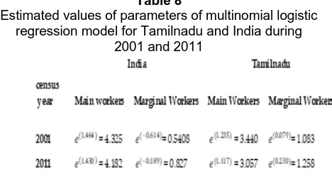
Table 8

Estimated values of parameters of multinomial logistic regression model for Tamilnadu and India during

2001 and 2011

From the above table it is observed the multinomial logistic regression models interpret that the odds of a migrant with main workers category increases of 432% in 2001 whereas in 2011 it increases 418% than the odds that a migrant be female for employment for India. According to marginal workers, the odds of a migrant category decreases of 46% in 2001 and in 2011 it also decreases in 18% respectively for India. Similarly, for Tamilnadu, the model interprets that the odds of a migrant with main workers category increases of 344% in 2001 whereas in 2011 it increases 305% than the odds that a migrant be female for employment. According to marginal workers, the odds of a migrant category increases of 108% in 2001 and in 2011 it also increases in 125% respectively.

5 CONCLUSIONS

The coefficients in a logistic regression are log odds ratios. Negative values mean that the odds ratio is smaller than 1, that is, the odds of the test group are lower than the odds of the reference group. In 2001 and 2011, using multiple logistic regression model shows duration of stay for male migrants as a risk factor which highly influence the

migration according to reasons (work/employment,

education, marriage etc.,) than female for both India and

Tamilnadu. In 2001, by using multinomial logistic regression model main workers category for employment having increased pattern in male migrants than female migrants for both India and Tamilnadu. According to marginal workers category there is an increasing trend in India and in Tamilnadu there is a decreasing trend for male migrants than female migrants. In 2011, male migrants of main workers category increase for migration in India but there is a decrease of migration pattern in Tamilnadu. In contrast, male migrants of marginal workers in India reveals an increased trend and in Tamilnadu there is a decreasing

trend for males than female for employment status. The

result shows marginal workers are lower than the non-workers compared with main non-workers in both India and Tamilnadu for the census years 2001 and 2011. Also, it is

observed that Migrants’ gender influences the probabilities

(6)

1336

REFERENCES

[1]

Christiane von Reichert and Gundars Rudzitis(1992),

―Multinomial Logistic models explaining income changes of migrants to high amenity counties‖, The review of journal studies, University o Idaho

[2] David W. Hosmer and Stanley Lemeshow(2000),

―Applied Logistic Regression‖, 2nd

edition, A Wiley-Interscience publication, John Wiley & sons, ISBN :0-471-35632-8.

[3] Jorge Garza-Rodriguez, Jennifer Fernandez-Ramos

and Ana K. Garcia-Guerra, Gabriela Morales-Ramirez(2015), ―The Dynamics of poverty in Mexico: A Multinomial logistic regression analysis‖, Universidad de Monterrey, MPRA paper No. 77743, April 2015.

[4] McCullagh, P. and Nelder, J. A.(1989), ―Generalized

linear models‖, Chapman & Hall, London.

[5] Nur Ain Abd Aziz, Zalila Ali, Norlida Mohd Nor, Adam

Baharum and Maizurah omar(2016), ―Modelling multinomial logistic regression on characteristics of smokers after the smoke free campaign in the Melaka Advances in Industrial and Applied Mathematics

(AIPConference Proceedings 1750,060020,

https://doi.org/1.4954625 ,

[6] June 21, 2016. Nurullah MD and MD.Rafiqul

Islam(2011), ―Determinants of socio- demoraphic

characteristics on female migrants: Logistic Regression model ‖, International Journal of Applied Mathematical Analysis and Applications, Vol. 6(1-2), pp.95-102.

[7] Pandey A.P(2016), ―Socio economic factors of contract

farming: A Logistic analysis‖,International Journal of Management & social sciences, ISSN 2455-2267,Vol 3(3).

[8] Singh S.K. and Urvashi Pandey(2017), ―A Logistic

analysis between Internal migration and the

development, A study of Almora District in Uttarakhand‖, International Research Journal of Commerce Arts and Science, Vol. 8(5), ISSN 2319-9202.

9] Zezula (2010), ―Logistic, multinomial, and ordinal regression‖, J.Safarik

University, Kosice.

[10] www.Censusindia.gov.in Office of the Registrar

General &