A multi-wavelength census of star formation at redshift z~2

(1)

z

∼

2

Thesis by Naveen A. Reddy

In Partial Fulfillment of the Requirements for the Degree of

Doctor of Philosophy

California Institute of Technology Pasadena, California

2006

(2)

ii

c

2006 Naveen A. Reddy

(3)

Acknowledgements

This thesis work, and the valuable experience I have gained as a graduate student at Caltech,

were made possible by more people than I can name here. During my first year at Caltech

the senior graduate students made us feel welcome and provided us with great insights into

the department and the faculty. I would like to thank Nick Scoville for making Caltech a

less intimidating place with his informal yet enthusiastic presence. Thanks to my former

collaborators in the world of long wavelength astronomy, including Nick, Andrew Blain,

Dave Frayer, and Lee Armus. I would especially like to acknowledge Lee for teaching me

the correct way to handle Keck ToO requests. Thanks to Shardha for her patience while

teaching me the ropes at OVRO.

I am grateful to the peers in my graduate class, especially Pranjal Trivedi, Alison Farmer,

Dawn Erb, and George Becker, for going through classes with me and sharing in the trials

and tribulations of graduate school. Thanks also to my regular lunch group, including

Micol Christopher, George, Edo Berger, Dawn, Alison, Dave Kaplan, and Jackie Kessler,

for providing a necessary respite during the middle of the day.

I am indebted to my former officemates, Dawn Erb, Alison Farmer, Jackie Kessler, Alicia

Soderberg, and Joanna Brown, for providing just the right amount of distraction to keep

me going throughout the day. A special acknowledgment goes out to Alison for keeping me

company in the office when no one else seemed to be around, and for our endless discussions

of Daleks and hemispherical bugs. And Jackie, for staying in the office late while working

on her thesis and accompanying me on trips to Baskin Robins to get a Chocolate Vortex.

And Alicia, both for keeping me company in the office and for keeping me apprised of who

was making all that noise outside our office.

A special thanks to the Astronomy Department systems administrators, Patrick

Shop-bell, Cheryl Southard, and Anu Mahabal, for always being ready with a solution whenever

my machine, nicmos, started acting up. They know more about computers than anyone

else I know, and my thesis work would not have been possible without their support. I am

grateful to the Caltech ITS technician, Kar Cheung, for tirelessly working for 6 straight

months to get my Mac laptop working again.

All of the work in this thesis is based on a spectroscopic sample of galaxies obtained

(4)

iv

for the best possible instrument support. Thanks to Jean Mueller and Karl Dunscombe for

their lively company during the long nights at Palomar, and Dipali and Rose for their good

cooking and hospitality at the Monastery.

I am lucky to have been a part of an excellent collaborative group, including Alice

Shapley, Max Pettini, Kurt Adelberger, Dawn Erb, and Matt Hunt. I especially want to

acknowledge Max for being a steadfast collaborator who always provided insightful

com-ments and suggestions, and great humor during observing runs and conferences. Kurt was

also an excellent resource of information and, while we did not overlap at Caltech, I am

grateful that he accompanied us on a few observing trips to Keck. And of course Dawn Erb,

who has been there since the beginning as a classmate, collaborator, and a good friend.

I would be amiss not to mention the support and encouragement of two very close friends,

Micol Christopher and Alice Shapley, whom I’ve come to think of as siblings. Thanks, Micol,

for being a loyal friend and a constant pillar of support for me through some tough times,

and for sharing in the good times. Thanks also for letting me bug you everyday to make

light conversation when I needed some distraction from work. And, of course, Alice, who

has been an unwavering source of enthusiasm, support, and encouragement, and with whom

I’ve had many conversations about galaxies, ramekins, and menudo, which kept me going

throughout the day.

I am grateful to Min Yun whose mentoring and friendship while I was a summer student

at NRAO prompted my decision to pursue astrophysics as a career. And, last but not least,

none of this would have been possible without my advisor, Chuck Steidel. Despite his busy

schedule, Chuck was always available to look at drafts of papers, send comments, suggest

new avenues to pursue, and answer my questions with patience. He provided just the

right amount of independence and encouragement. I also particularly enjoyed the scientific

discussions I had with Chuck. Chuck is an easy person to work with; his approachability

and modesty are only superseded by his incredible grasp of astronomy, and he is one of the

smartest people I know. I am very grateful to have had the opportunity to be his graduate

student. Finally, I could not have come this far without the support and encouragement of

(5)

A Multi-Wavelength Census of Star Formation at Redshifts z ∼ 2 by

Naveen A. Reddy

In Partial Fulfillment of the

Requirements for the Degree of

Doctor of Philosophy

Abstract

We examine the census of star-forming galaxies and their extinction properties at redshift

z _∼ 2, when a large fraction of the stellar mass in the universe formed. We find a good agreement between the X-ray, radio, and de-reddened UV estimates of the average star

formation rate (SFR) for our sample ofz_∼2 galaxies of_∼50M⊙ yr−1, indicating that the

locally calibrated SFR relations appear to be statistically valid from redshifts 1.5_∼< z_∼<3.0.

Spitzer MIPS data are used to assess the extinction properties of individual star-forming

galaxies, and we find that the rest-frame UV slope of most galaxies at z _∼2 can be used to infer their attenuation factors, Lbol/LUV. As in the local universe, the obscuration,

LFIR/LUV, is strongly dependent on bolometric luminosity, and ranges in value from < 1

to _∼ 1000 within the sample considered. However, the obscuration is _∼ 10 times smaller

at a given Lbol (or, equivalently, a similar level of obscuration occurs at luminosities ∼10

times larger) at z_∼2 than at z_∼0. This trend is expected as galaxies age and their gas becomes more dust-enriched. Specific SFRs indicate wide range in the evolutionary state

of galaxies at z _∼ 2, from galaxies that have just begun to form stars to those that have already accumulated most of their stellar mass and are about to become, or already are,

passively evolving. Finally, we examine two techniques for assessing the census of galaxies

at z _∼2. In the first, we select galaxies using optical, near-IR, and sub-mm criteria, and find a large overlap between optical and near-IR selected samples of galaxies at z _∼ 2. The second technique involves reconstructing the luminosity function of z _∼2 galaxies as determined from Monte Carlo simulations. We find that the SFR density increases between

(6)

vi

(7)

List of Figures

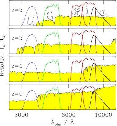
1.1 UnGRIz Colors of Galaxies at 0< z <3 . . . 5

1.2 ExpectedUnGRColors of Star-Forming Galaxies . . . 6

1.3 Spectroscopic Redshift Distributions . . . 8

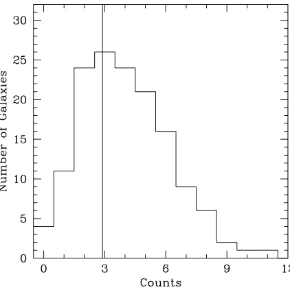
2.1 Average X-ray Count Distribution . . . 16

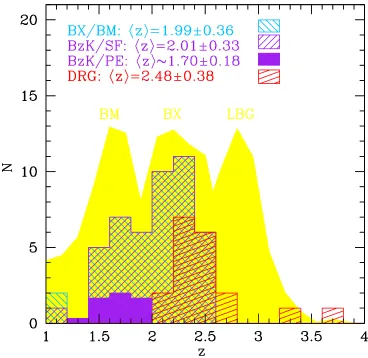
3.1 Spectroscopic Redshift Distributions to Ks= 21 . . . 28

3.2 Redshift Distribution of BzK Galaxies . . . 30

3.3 Transmission of z,J,Ks, and IRAC 3.6 µm Filters . . . 32

3.4 Optical Magnitude Distributions . . . 33

3.5 Optical/X-ray Flux Ratios . . . 36

3.6 IRAC Colors . . . 38

3.7 z₋K Color Distribution . . . 40

3.8 (z₋K)ABversus Optical Magnitude . . . 41

3.9 J ₋Ks Color Distributions . . . 42

3.10 Overlap Fraction Between Optical/Near-IR Samples . . . 43

3.11 BX/BM Colors of BzK Galaxies . . . 44

3.12 BzK Colors of BX/BM Galaxies . . . 46

3.13 BzK Colors as a Function of Ks . . . 48

3.14 Stacked X-ray Luminosity as a Function of Ks . . . 51

3.15 X-ray Inferred Star Formation Rates . . . 53

3.16 Variation of SFR with Near-IR Color . . . 56

3.17 Attenuation Distribution with Near-IR Color . . . 57

3.18 Comparison of Colors with SED Models . . . 63

(12)

xii

3.20 Cumulative Star Formation Rate Density . . . 70

4.1 Redshift Distribution of Optical/Near-IR Samples . . . 90

4.2 Expected 24 µm Fluxes of Local Templates . . . 94

4.3 Photo-z Results . . . 95

4.4 Ratio of Mid-IR to X-ray Luminosity . . . 99

4.5 Comparison Between MIPS and Hα InferredLbol . . . 102

4.6 Distributions of LIR . . . 103

4.7 L850_IRµm versusL5_IR−8.5µm . . . 107

4.8 LIR as a Function of Near-IR Magnitude and Color . . . 108

4.9 Stacked 24 µm Flux of MIPS-Undetected Galaxies . . . 110

4.10 IRX-β Relation atz_∼2 . . . 114

4.11 Lbol versus Dust Obscuration . . . 119

4.12 Histograms of Age and Mass . . . 122

4.13 Normalized Composite UV Spectra . . . 124

4.14 Lbol versus Stellar Mass . . . 126

4.15 Specific Star Formation Rate . . . 132

5.1 Positions of BX/BM Galaxies in GOODS-N Field . . . 147

5.2 BX/BM Color Selection Windows . . . 149

5.3 Redshift Histograms for BM/BX and LBG Galaxies . . . 153

5.4 Stellar Mass Distribution of BX/BM Galaxies . . . 158

5.5 SEDs of Obscured AGN . . . 162

6.1 Redshift Distribution of BX Galaxies . . . 225

6.2 Perturbation of BX/BM colors from Lyα . . . 226

6.3 Apparent Magnitude versus Redshift . . . 228

6.4 Lyα Equivalent Width Distributions . . . 232

6.5 Transitional Probability Function . . . 238

6.6 Expected and Observed Redshift Distributions . . . 240

6.7 Best-fit E(B₋V) Distribution . . . 241

6.8 E(B₋V) Distribution in Bins of Apparent Magnitude . . . 244

(13)

6.10 Covariance Between α and M∗

. . . 248

6.11 Degeneracy Between Schechter Parameters . . . 249

6.12 Dispersion in LF Normalization . . . 251

6.13 Attenuation as a Function of Apparent Magnitude . . . 254

6.14 Comparison of z_∼2 and z_∼3 E(B₋V) Distributions . . . 256

(14)

xiv

List of Tables

2.1 Radio and X-ray Stacking Results . . . 19

2.2 Star Formation Rate Estimates . . . 20

3.1 Interloper Contamination of the BX/BM Sample . . . 76

3.2 Sample Properties . . . 77

3.3 Possible Star-Forming Direct X-ray Detections . . . 79

3.4 Properties of Submillimeter Galaxies with Ks-band Data . . . 80

3.5 Cumulative Contributions to the SFRD Between 1.4< z <2.6 . . . 82

4.1 Properties of the Samples . . . 138

4.2 Local Template Galaxies . . . 139

4.3 Interstellar Absorption Line Wavelengths and Equivalent Widths for 24µm Detected and Undetected BX/BM Galaxies . . . 140

5.1 Sample Statistics to _R= 25.5 . . . 165

5.2 GOODS-N BX/BM Galaxies with Spectroscopic Redshifts . . . 166

5.3 Spitzer Photometry . . . 187

5.4 Stellar Population Parameters . . . 200

5.5 Stellar Masses . . . 214

5.6 AGN at z >1.4 . . . 215

6.1 Survey Fields . . . 261

(15)

Chapter 1

Introduction

Understanding the star formation history and stellar mass evolution of galaxies is perhaps

one of the most fundamental issues in cosmology. Observations of the stellar mass and

star formation rate density, the number density of QSOs, and galaxy morphology at both

low (z _∼< 1) and high (z _∼> 3) redshifts indicate that most of the activity responsible for shaping the bulk properties of galaxies to their present form occured in the epochs between

1_∼< z _∼<3 (e.g., Dickinson et al. 2003b; Rudnick et al. 2003; Chapman et al. 2005; Madau et al. 1996; Lilly et al. 1996, 1995; Steidel et al. 1999; Shaver et al. 1996; Fan et al. 2001; Di

Matteo et al. 2003; Conselice et al. 2004; Papovich et al. 2003; Shapley et al. 2001; Giavalisco

et al. 1996). Galaxy studies during this intermediate redshift range have suffered, however,

because of our inability to identify large samples of galaxies during this critical epoch. The

primary difficulty at these redshifts was due to the fact that the lines used for redshift

identification are shifted into the near-UV where detector sensitivity has lagged, or to the

near-IR where spectroscopy is more difficult due to higher backgrounds.

However, the advent of 8₋10 m class telescopes and improvements in detector technology

have allowed us to make significant progress by making it possible to select large samples

of galaxies during the critical epochs corresponding to redshifts 1.4 _∼< z _∼<3.0. There are essentially two ways in which to proceed in order to assess the census of galaxies at high

redshift. The first is to observe galaxies over as wide a range in wavelengths as possible

in order to select those that comprise the bulk of the total star formation rate density

(SFRD). Along this line, several color criteria have been developed to target galaxies over

(16)

2

2004; Steidel et al. 2004). The second method is to select galaxies by their near-IR z₋K

color, taking advantage of the fact that for redshiftsz_∼>1.4, the z₋and K-bands bracket the age-sensitive Balmer and 4000 ˚A break features in the spectra of most star-forming and

“passively evolving” (or quiescent) galaxies (Daddi et al. 2004b). The third method selects

either passively evolving or star-forming galaxies at redshifts z _∼> 2 based on the single color criteriaJ₋Ks >2.3 (in Vega magnitudes), again taking advantage of the Balmer and

4000 ˚A breaks (Franx et al. 2003). The fourth method relies on the monochromatic flux

at 850µm to select dusty, high redshift galaxies (Blain et al. 1999). Each selection method presents its own advantages and disadvantages, but one critical issue that has previously

been neglected is that one must take into account the substantial overlap between these

samples when estimating the total SFRD (Reddy et al. 2005). Each of the selection criteria

and their respective overlap and contributions to the SFRD are discussed in Chapter 3.

The second approach to assessing the total star formation rate density is to simulate

many realizations of the intrinsic distribution of galaxy properties at high redshift, subject

these realizations to the same photometric methods and selection criteria as applied to real

data, and then adjust the simulated realizations until convergence is reached between the

expected and observed distribution of galaxy properties. This Monte Carlo approach has

the advantage, unlike the first method, of not requiring the observational effort necessary

to conduct a panchromatic assessment of the total SFRD. The method works especially

well when applied to joint spectroscopic and photometric samples of galaxies and therefore

works best for optically-selected samples where spectroscopy is much more feasible than for

near-IR selected samples. Perhaps the main disadvantage of this method is the inability

to correct sample completeness for galaxies that are completely missed (i.e., not scattered

into the color selection windows). Nevertheless, applying this method to spectroscopically

confirmed samples of high redshift galaxies allows one to evaluate the systematic effects of

photometric scatter and the intrinsic variation in colors due to line emission and absorption

with great accuracy. We can further evaluate the signficance and magnitude of the dust

extinction corrections necessary to translate UV luminosities to total bolometric luminosities

(see below and Chapters 2, 3, 4, and 6). Our Monte Carlo approach to computing sample

incompleteness can then be used to reconstruct the total SFRD. This method is discussed

(17)

1.1

The Optical Selection of High Redshift Galaxies

1.1.1 Photometric Selection

Constructing a practical set of selection criteria to select all galaxies in any desired redshift

range and reject all others is an intractable problem. One extreme is to select all objects

down to a given magnitude limit, such as in flux-limited surveys of high redshift galaxies,

but unfortunately such studies suffer from significant amounts of foreground contamination.

Without additional color criteria, one may spend 99% of the time spectroscopically

con-firming low redshift contaminants before assembling a significant sample of galaxies at the

desired redshift range. Color-selected samples have the distinct advantage of allowing one

to specifically target a desired redshift range while minimizing the number of interlopers.

Perhaps the most successful of the various color criteria that have been designed to select

galaxies at different epochs is rest-frame UV color selection, pioneered by Steidel et al.

(1995) to select galaxies at z _∼ 3, and extended to higher redshifts (e.g., Bouwens et al. 2005, 2004; Bunker et al. 2004; Dickinson et al. 2004; Yan et al. 2003). The success of this

technique is partly due to its simplicity in that only a few broadband filters are required

to assemble such samples and, at lower redshifts (1.4 _∼< z _∼< 3.5), where the galaxies can be spectroscopically observed and precise redshifts can be obtained in a short amount of

observing time. Combined, these surveys have given us an unprecedented view of galaxy

evolution over almost the entire age of the universe.

For the past several years, the main focus of our group has been to assemble a large

sam-ple of galaxies at the peak epoch of galaxy formation and black hole growth, corresponding

to redshifts 1.5_∼< z_∼<2.6. The selection criteria aim to select actively star-forming galaxies at z_∼2 with the same range in intrinsic UV color and extinction as Lyman break galaxies (LBGs) atz_∼3 (Steidel et al. 2003). While galaxies atz_∼2 do not have any of the strong spectral breaks across theUnGRbands used to select higher redshift galaxies (Figure 1.1), they do occupy a particular area ofUnGRcolor space that can be singled out (Figure 1.2). We have used the “BX” criteria of Adelberger et al. (2004) and Steidel et al. (2004) to

(18)

4

colors:

G_{− R ≥ −}0.2

Un−G ≥ G− R+ 0.2

G_{− R ≤} 0.2(Un−G) + 0.4

Un−G ≤ G− R+ 1.0. (1.1)

Similarly we have selected “BM” galaxies at redshifts 1.5 _∼< z _∼< 2.0 using the following criteria:

G_{− R ≥ −}0.2

Un−G ≥ G− R −0.1

G_{− R ≥} 0.2(Un−G) + 0.4

Un−G ≤ G− R+ 0.2. (1.2)

To ensure a sample of galaxies amenable to spectroscopic followup, we imposed a magnitude

limit of _R= 25.5. This limit corresponds to an absolute magnitude 0.6 mag fainter atz= 2.2_±0.4 (the mean and dispersion of the measured redshift distribution for BX candidates with z > 1) than at z _∼ 3. We also excluded candidates with _R < 19 since almost all of these objects are stars. Given the constraints of the color criteria and the self-imposed

magnitude limits, the combined BM, BX, and LBG samples constitute 25 to 30% of the

total _R andKs band counts to R= 25.5 and Ks(AB) = 24.4, respectively.

1.1.2 Spectroscopic Followup

The spectroscopic followup to the optically selected sample is discussed in detail in the

following chapters. Briefly, we took advantage of the multi-object capabilities of the Keck

LRIS (Low Resolution Imaging Spectrograph; Oke et al. 1995) instrument to obtain

spec-troscopy. The unrivaled near-UV sensitivity of the blue arm of LRIS (LRIS-B; Steidel et al.

2004) is necessary for spectroscopically identifying galaxies in the so-called spectroscopic

desert where BX and BM selected galaxies are expected to lie and where the stellar and

(19)

(20)

6

Figure 1.2 Expected UnGR colors of stars (stars; from Gunn & Stryker 1983) and star-forming galaxies at redshifts z = 1.5, 2.0, and 2.5 (blue circles and red squares; data from Papovich et al. 2001 and Shapley et al. 2001). Green tracks indicate the colors of

galaxies of different spectral types (Im, Sb, Sc), proceeding from z = 0 to z = 1.5, in intervals of δz = 0.1 as denoted by the crosses. The trapezoid denotes the BX selection window, as defined by Equation 1.1, which is designed to include as many galaxies at

(21)

near-UV. The spectroscopic sample presently consists of 104 BM, 1125 BX, and 1444 LBG

galaxies (spread throughout multiple uncorrelated fields), with mean spectroscopic redshifts

of _hz_i = 1.72_±0.34, _hz_i = 2.20_±0.32, and _hz_i = 2.96_±0.26, for the BM, BX, and LBG samples, respectively (Figure 1.3). It is the spectroscopic samples at z_∼2 (BM and BX) that form the basis of the work presented in Chapters 2, 3, 4, and 5. In Chapter 6, we

con-sider the joint photometric and spectroscopic samples to compute the luminosity function

and the contribution of optically-selected galaxies to the total star formation rate density

at z_∼2.

1.2

Bolometric Measures of Star Formation Rates

Estimating the star formation rates of galaxies based on a single monochromatic flux (or

even broadband SEDs) entails many assumptions, some of which have been tested and

oth-ers which have not. For example, one must assume a particular form of the initial mass

function (IMF) of stars in order to estimate a star formation rate, but directly measuring

the IMF is very difficult for everything except local global clusters where stars can be

in-dividually resolved. Another assumption that was previously untested at high redshift is

the relationship between the observed UV luminosities of star forming galaxies and their

total bolometric luminosities. Prior to the advent of large-scale multi-wavelength surveys,

it was common to make untested extinction corrections to galaxies in UV surveys based on

relationships established locally. The situation has changed significantly with panchromatic

surveys which have allowed us to examine the extinction free measures of star formation

rates in high redshift galaxies and compare these estimates with the observed UV emission,

as discussed in Chapters 2 and 4. Combining our census of the star-forming galaxy

popu-lation at high redshift and our intimate knowledge of the extinction corrections required to

estimate bolometric SFRs, we can now make assertions regarding the star formation

his-tory and buildup of stellar mass in the Universe with much more confidence than previously

(22)

8

Figure 1.3 Arbitrarily normalized spectroscopic redshift distributions of galaxies with z >

(23)

1.3

Outline of the Thesis

The outline of this thesis is as follows. In the next chapter, we use deep X-ray and radio

emission as independent probes of the star formation rates and bolometric activity in

galax-ies at z _∼2. While the X-ray and radio data are not sufficiently sensitive to detect most optically-selected galaxies at these redshifts, we can use stacking analyses to infer

impor-tant information regarding the average star formation rates of well-selected subsamples of

galaxies. In Chapter 3, we perform a detailed comparison of galaxies selecting using optical,

near-IR, and sub-mm criteria. We quantify the overlap between these samples and, using

stacked X-ray emission, demonstrate that this sample overlap must be taken into account

when estimating the total star formation rate density. We extend the results of the

cen-sus of star-forming galaxies presented in Chapter 3 by examining the rest-frame infrared

emission from z _∼ 2 galaxies selected in various ways. We also discuss how the average extinction factors for galaxies of a given luminosity change as a function of redshift, from

z_∼2 to z = 0. We go on to show how bolometric measures of the star formation rates of galaxies, combined with stellar mass estimates from population synthesis modelling, can be

used to deduce the evolutionary state of galaxies in terms of their propensity for future star

formation. In Chapter 5 we discuss in detail the spectroscopic sample of optically-selected

galaxies in the GOODS-North field (Giavalisco et al. 2004b; Dickinson et al. 2003a), which

is the basis for the work presented in Chapters 2, 3, and 4. Using multi-wavelength data in

this field, we examine the properties of obscured AGN in optically-selected host galaxies.

Finally, in Chapter 6, we use sophisticated Monte Carlo analysis of our joint photometric

and spectroscopic samples of galaxies in the z _∼ 2 survey (e.g., Adelberger et al. 2004; Steidel et al. 2004) to estimate the effects of photometric scattering, Lyman-alpha line

per-turbations, and other systematic effects introduced by the optical selection of star-forming

galaxies at redshift z _∼ 2. We use these results to construct the luminosity function at

z_∼2, and incorporating our knowledge of extinction, to estimate the total star formation rate density and the implications for the star formation history and buildup of stellar mass

in the Universe. Finally, in the epilogue, we discuss several unresolved but important

is-sues to consider for obtaining even more stringent constraints on the cosmic star formation

(24)

10

Chapter 2

X-Ray and Radio Emission from UV-Selected Star

Forming Galaxies at Redshifts 1

.

5

∼

< Z

∼

<

3

.

0 in

the GOODS-North Field

∗†

Naveen A. Reddy & Charles C. Steidel

California Institute of Technology, MS 105–24, Pasadena, CA 91125; [email protected],

[email protected]

Abstract

We have examined the stacked radio and X-ray emission from UV-selected galaxies

spec-troscopically confirmed to lie between redshifts 1.5_∼< z_∼<3.0 in the GOODS-North field to determine their average extinction and star formation rates (SFRs). The X-ray and radio

data are obtained from the Chandra 2 Msec survey and the Very Large Array, respectively.

There is a good agreement between the X-ray, radio, and de-reddened UV estimates of the

average SFR for our sample ofz_∼2 galaxies of_∼50 M⊙ yr

−1_{, indicating that the locally}

calibrated SFR relations appear to be statistically valid from redshifts 1.5 _∼< z_∼<3.0. We find that UV-estimated SFRs (uncorrected for extinction) underestimate the bolometric

∗_{Based on data obtained at the W. M. Keck Observatory, which is operated as a scientific partnership}

among the California Institute of Technology, the University of California, and NASA, and was made possible

by the generous financial support of the W. M. Keck Foundation.

(25)

SFRs as determined from the 2 to 10 keV X-ray luminosity by a factor of _∼4.5 to 5.0 for galaxies over a large range in redshift from 1.0_∼< z_∼<3.5.

2.1

Introduction

Estimating global star formation rates (SFRs) of galaxies typically requires using relations

that can be quite uncertain as they incorporate a large number of assumptions in

convert-ing between specific and bolometric luminosities (e.g., assumed IMF, extinction, etc.; e.g.,

Adelberger & Steidel 2000). The varied efforts in the Great Observatories Origins Deep

Survey (GOODS; Giavalisco et al. 2004b) allow us to examine the same galaxies over a

broad range of wavelengths to mitigate some of these uncertainties. X-ray, radio, and UV

emission are all thought to result directly from massive stars and are consequently used as

tracers of current star formation (e.g., Ranalli et al. 2003; Condon 1992; Gallego et al. 1995).

Here we use the X-ray, radio, and UV emission, each differently affected by extinction (or

not at all), to determine SFRs of galaxies at z_∼2.

Observations of the QSO and stellar mass density, and morphological diversification all

point to the epoch around z_∼2 as an important period in cosmic history (e.g., Di Matteo et al. 2003; Chapman et al. 2003). Until recently, this epoch has been largely unexplored as

lines used for redshift identification are shifted to the near-UV, where detector sensitivity has

been poor or to the near-IR, where spectroscopy is more difficult due to higher backgrounds.

With the recent commissioning of the blue side of the Low Resolution Imaging Spectrograph

(LRIS; Oke et al. 1995) on the Keck I telescope, we have for the first time been able to obtain

spectra for large numbers of galaxies at these redshifts. Adding to the multi-wavelength

efforts in the GOODS-North field, we have undertaken a program to identify photometric

candidates in this field between 1.5 _∼< z _∼< 3.0 and perform followup spectroscopy with LRIS-B (Steidel et al. 2004). This UV-selected sample of galaxies forms the basis for our

subsequent multi-wavelength analysis.

Current sensitivity limits at X-ray and radio wavelengths preclude the direct detection

of normal star forming galaxies atz_∼>1.5. Nonetheless, we can use a “stacking” procedure to add the emission from a class of objects in order to determine their average emission

properties (e.g., Nandra et al. 2002; Brandt et al. 2001; Seibert et al. 2002). In this paper,

(26)

12

galaxies at redshifts 1.5 _∼< z _∼< 3.0 to cross-check three different techniques of estimating SFRs at high redshifts. Ho = 70 km s−1 Mpc−1, ΩM = 0.3, and ΩΛ = 0.7 are assumed

throughout.

2.2

Data

The techniques for selecting galaxies at z_∼2 are designed to cover the same range of UV properties and extinction to those used to select Lyman-break galaxies (LBGs) at higher

redshifts (z _∼> 3.0; Adelberger et al. 2004). Here, we simply mention that we have two spectroscopic samples at 1.5_∼< z_∼<2.5: a “BX” sample of galaxies selected on the expected

UnGR colors of LBGs de-redshifted to 2.0 _∼< z _∼< 2.5; and a “BM” sample targeting

z _∼1.5₋2.0. (see Adelberger et al. 2004; Steidel et al. 2004 for a complete description). We presently have 138 redshifts (_hz_{i ∼}2.2_±0.3) and 48 redshifts (_hz_{i ∼} 1.7_±0.3) in the GOODS-North BX and BM samples, respectively.

The X-ray data are from the Chandra 2 Msec survey of the GOODS-North region

(Alexander et al. 2003). We made use of their raw images and exposure maps in the Chandra

soft X-ray band (0.5₋2.0 keV). Dividing the raw image by the appropriate exposure map yields an image with the count rates corrected for vignetting, exposure time, and variations

in instrumental sensitivity. The on-axis soft band sensitivity is_∼2.5_×10−₁₇

ergs cm−₂

s−₁

(3 σ).

The radio data are from the Richards (2000) Very Large Array (VLA) survey of the

Hubble Deep Field North (HDF-N), reaching a 3 σ sensitivity of _∼ 23µJy beam−1 _at

1.4 GHz. The final naturally weighted image has a pixel size of 0′′.

4 and resolution of 2′′.

0,

with astrometric accuracy of<0′′.

03.

2.3

Stacking Procedure

We divided the spectroscopic data into subsets based on selection (BX and BM) and redshift,

removed sources with matching X-ray or radio counterparts within 2′′.

5 (or sources whose

apertures are large enough to contain emission from a nearby extended X-ray or radio

source), and stacked galaxies in these subsets. Four of the removed x-ray/radio sources are

(27)

The X-ray data were stacked using the following procedure. We added the flux within

apertures randomly dithered by 0′′.

5 at the positions of the galaxies (targets) in the X-ray

images to produce a signal. Similarly sized apertures were randomly placed within 5′′

of

the galaxy positions to sample the local background near each galaxy while avoiding known

X-ray sources. This was repeated 1000 times to estimate the mean signal and background.

The Chandra PSF widens for large angles from the average pointing (off-axis angle), and

we fixed the aperture sizes to the 50% encircled energy (EE) radii (Feigelson et al. 2002)

for off-axis angles > 6′

. Background included at large off-axis angles becomes significant

due to increasing aperture size and this can degrade the total stacked signal. Consequently,

we only stacked galaxies within the off-axis angle that results in the highest S/N (this

varies for each subsample, from 6 to 8′

). Including all sources in the stack reduces the

S/N but does not affect the absolute flux value. For sources<6′

from the pointing center,

the 50% EE radius falls below 2′′.

5, and we adopted a fixed 2′′.

5 radius aperture to avoid

the possibility of placing an aperture off a target as a result of dithering or astrometric

errors—which are _∼ 0′′.

3—for sources very close to the average pointing. Stacking was

performed on both the raw and normalized images to calculate the S/N and total count

rate, respectively. Aperture corrections were applied to the raw counts and count rate. The

conversion between count rate and flux was determined by averaging the count rate to flux

conversions for the 74 optically bright X-ray sources in Table 7 of Alexander et al. (2003)

that are assumed to have a photon index of Γ = 2.0, typical of the X-ray emission from star forming regions (e.g., Kim et al. 1992; Nandra et al. 2002), and incorporate corrections

for the QE degredation of the ACIS-I chips. In converting flux to rest-frame luminosity, we

assume Γ = 2.0 and a Galactic absorption column density ofNH= 1.6×1020 cm−2 (Stark

et al. 1992). Uncertainties in flux and luminosity are dominated by Poisson noise and not

the dispersion in measured values for each stacking repetition, so we assume the former.

To stack the radio data, we extracted subimages at the locations of the targets from

the mosaicked radio data of Richards (2000). These were corrected for the primary beam

attenuation of the VLA with a maximum gain correction of 15%, coadded using a 1/σ2

weighted average to produce a stacked signal with maximal S/N _∼4.5, and smoothed by 1′′.

(28)

14

AIPS1 task JMFIT using an elliptical gaussian to model the stacked emission. We assume

a synchrotron spectral index of γ =₋0.8, typical of the non-thermal radio emission from star-forming galaxies (Condon 1992). Results of the X-ray and radio stacks for various

subsamples are presented in Table 2.1. Four subsamples contain too few sources to yield a

robust estimate of the stacked radio flux.

2.4

Results and Discussion

2.4.1 SFR Estimates

The relations established atz= 0 to convert luminosities to SFRs for ourz_∼2 sample are adopted from the following sources: Kennicutt (1998a,b) for conversion of the 1500₋2800 ˚A

luminosity; Ranalli et al. (2003) for the 2₋10 keV luminosity; and Yun et al. (2001) for the

1.4 GHz luminosity. These relations must be used with caution when applied to individual galaxies given uncertainties in the SFR relations (e.g., burst age, IMF) as well as the factor

of _∼2 dispersion in the correlations between different specific luminosities. However, they

should yield reasonable results when applied to an ensemble of galaxies, as we have done

here.

Table 2.2 shows the SFR estimates based on the 2 ₋10 keV (“SFRX”), 1.4 GHz

(“SFR1.4 GHz”), and UV (“SFRUV”) luminosities, with typical error of ∼ 20%. We

ap-proximate the UV luminosity by using the 1600 ˚A rest-frame flux for all samples except

the highest redshift bin sample (2.5 < z _∼< 3.0) where we use the 1800 ˚A rest-frame flux. UV-estimated SFRs were corrected for extinction using the observedG_{− R} colors, a spec-tral template assuming constant star formation for>108 yr (after which the UV colors are essentially constant), and applying the reddening law of Calzetti et al. (2000) and Meurer

et al. (1999). We created four additional subsamples of galaxies according to de-reddened

UV-estimated SFR, also shown in Table 2.2.

1_{AIPS is the Astronomical Image Processing System software package written and supported by the}

(29)

2.4.2 Stacked Galaxy Distribution and AGN

Stacking only indicates the average emission properties of galaxies, not their actual

distri-bution, and the observed signal may result from a few luminous sources lying just below

the detection threshold. To investigate this, we plot the average distribution in counts for

the sample of 147 stacked spectroscopic galaxies (Figure 2.1). Much of the high-end tail of

the distribution results from random positive fluctuations. Only three sources consistently

had >7 counts. Removing those objects whose apertures have>6 counts still results in a stacked signal with S/N _∼2.5 and an average loss of 21 galaxies (_∼14% of the sample). It is therefore likely that most of the stacked galaxies contribute to the signal, particularly

given their wide range in optical, and likely X-ray, properties.

Contribution of low luminosity AGNs to the stacked signal is a concern. This is a

problem with most X-ray stacking analyses, but we also possess the UV spectra for our

sources. There are two objects undetected in X-rays for which the UV spectra show emission

lines consistent with an AGN. Our ability to identify AGNs from their UV spectra regardless

of their X-ray properties, and having identified only 2 such objects out of 149, suggests that

subthreshold luminous AGNs do not contribute significantly to the stacked X-ray flux.

Furthermore, UV selection biases against the dustiest sources so we do not expect to find

many Compton-thick AGNs in our sample.

There are also two BM galaxies coincident with known radio sources that are not

de-tected in X-rays and are not included in the stacked samples. Removing such objects

ensures excluding radio-loud AGN that might have unassuming UV and X-ray properties.

For comparison, the 3σ radio sensitivity is sufficient to detect SFR_∼>170 M⊙yr−1, a factor

of 4 higher than the median SFR of our sample based on the X-ray or de-reddened UV

SFR estimates. The stacked X-ray emission indicates a SFR of_∼42 M⊙ yr−1. The on-axis

soft-band flux limit implies a sensitivity to SFR_∼> 186 M⊙ yr

−1 _at _z _∼_{2, a factor of 4}_.₅

higher than the average SFR for spectroscopic z _∼2 galaxies. Stacking the radio flux for the full spectroscopic sample indicates average SFRs from 33₋70 M⊙ yr

−1 _{depending on}

which estimator is used: the Bell (2003), Condon (1992), and Yun et al. (2001) calibrations

give low, high, and median (_∼ 56 M⊙ yr

−1_{) values, assuming} _γ ₌₋₀_._{8. We adopted the}

Yun et al. (2001) calibration as it is most relevant to the radio luminosity range considered

(30)

16

Figure 2.1 Average distribution of counts for the spectroscopic sample. The vertical line

denotes the average background count per aperture. The number excess at high counts

(31)

2.4.3 Bolometric Properties of z ∼ 2 Galaxies

The UV-implied reddening indicates AV ∼0.5 mag and NH ∼7.5×1020 cm−2 assuming

the Galactic calibration (Diplas & Savage 1994). For this column density, absorption in

the 2₋10 keV band is negligible, and we therefore assume that SFRX is indicative of the

bolometric SFR. In this case, we find a good agreement between the SFRs determined from

the X-ray, radio, and de-reddened UV luminosities (LX,L1.4 GHz, andLUV), suggesting that

the locally calibrated relations between specific luminosity and SFR remain valid within

the uncertainties at z _∼2, under the caution that we cannot independently test for these relations as we have no direct measure of Lbol.

The _hL_Xi and _hL1.4 GHzi of spectroscopically identified z ∼2 galaxies are comparable to those of local starbursts. The X-ray/FIR relation for local galaxies (Ranalli et al. 2003)

implies _hL_{FIRi ∼} 2.6 _×1011 L⊙. The stacked L₁_._{4 GHz} implies hLFIRi = 1.1×1011 L⊙

(Yun et al. 2001). These estimates are similar to the FIR luminosity of luminous infrared

galaxies (LIRGs), and are expected to have S850µm ∼ 0.3 mJy (e.g., Webb et al. 2003)

and would therefore be missing in confusion-limited SCUBA surveys to 2 mJy. Spitzer

will have the same rest-frame 7 µm sensitivity to z _∼ 2 galaxies as ISO has at z _∼ 1 for

LFIR _∼>5×1010 L⊙ galaxies (Weedman et al. 2004; Flores et al. 1999). Therefore, unlike

the stacked averages presented here, theSpitzerdata will be the first extinction-free tracer

of the SFR distribution of thez_∼2 sample as the stacked galaxies should be individually detected at 24µm.

For a fair comparison between the three redshift bins for 1.5< z_∼<3.0, we have added back those direct X-ray detections in the stacks for the 1.5 < z _≤ 2.0 and 2.0 < z _≤ 2.5 samples that would not have been detected if they hadz >2.5. There were no such sources with 1.5 < z _≤ 2.0 and only one with 2.0 < z _≤ 2.5, increasing _hL2−10 keVi by 2% to

2.38_×1041 ergs s−1_.

The distance independent ratio SFRX/SFRuncorUV (Table 2.2) is similar among the

selec-tion and redshift subsamples indicating that on average UV-estimated SFRs (uncorrected

(32)

18

BX/BM sample using the Calzetti et al. (2000) extinction law is similar to that computed

from SFRX/SFRuncorUV . The de-reddened UV-estimated SFRs (SFRcorUV) agree well with those

predicted from the radio continuum for the two samples for which radio estimates could be

obtained. Finally, we note the factor of_∼5 UV attenuation is similar to that advocated by

Steidel et al. (1999) for UV-selected samples at all redshifts.

The average attenuation factor increases as the SFR increases, as shown by the last four

subsamples in Table 2.2, and is expected if galaxies with higher SFRs have greater dust

content on average (Adelberger & Steidel 2000). SFRcor

UV follows the bolometric SFR even

for low luminosity systems, indicating that the observed correlations are not entirely driven

by only the most luminous galaxies.

2.5

Conclusions

We have made significant progress in estimating and comparing SFRs determined from

UV, X-ray, and radio emission from galaxies between redshifts 1.5 _∼< z _∼< 3.0, postulated to be the most “active” epoch for galaxy evolution. The locally calibrated SFR relations,

though uncertain in individual systems, appear to remain statistically valid at high redshift.

Stacking the X-ray and radio emission from UV-selected galaxies at z _∼ 2 indicates that these galaxies have an average SFR of_∼50 M⊙yr

−₁

and an average UV attenuation factor

of _∼ 4.5. The prospect of increased radio sensitivity with the E-VLA, as well as X-ray campaigns in different fields to similar depth as the 2 Msec survey in the GOODS-North

field, will allow for a more direct probe of the radio and X-ray flux distribution for the

stacked galaxies. SpitzerMIPS 24µm data for the GOODS-N field will trace the dusty star formation inz_∼2 galaxies and allow for the cross-checking of the results presented here.

We thank Alice Shapley, Dawn Erb, Matt Hunt, and Kurt Adelberger for help in

ob-taining the data presented here. CCS has been supported by grants AST 0070773 and

0307263 from the National Science Foundation (NSF) and by the David and Lucile Packard

(33)

19

F0.5−2.0 keVd L2.0−10 keVe S1.4 GHzf L1.4 GHzg νLνh

Sample Nsa hzib S/Nc (×10−18ergs cm−2 s−1) (×1041 ergs s−1) (µJy) (×1022 W Hz−1) (×1010L⊙)

BX+BM 147 2.09 8.9 5.65±0.68 2.11±0.25 2.30±0.65 5.90±1.66 3.50

BX 109 2.22 6.8 4.83±0.79 2.09±0.34 2.09±0.75 6.17±2.21 3.86

BM 38 1.71 6.0 8.04±1.34 1.84±0.31 ... ... 2.46

1.5< z≤2.0 54 1.82 5.6 6.89±1.27 1.84±0.33 ... ... 2.81 2.0< z≤2.5 73 2.24 6.0 5.24±0.96 2.33±0.43 ... ... 4.05 2.5< z≤3.0 43 2.87 3.3 4.21±1.46 3.40±1.18 ... ... 4.61

a_{Number of galaxies stacked}

b_{Mean redshift}

c_{Signal-to-noise calculated in a manner analogous to that in Nandra et al. 2002}

d_{Average soft-band X-ray flux per object}

e_{Average rest-frame X-ray luminosity per object, assuming Γ = 2}_._{0 and}_N

H= 1.6×1020cm−2, for our adopted cosmology f_{Average integrated radio flux density per object}

g_{Average rest-frame 1.4 GHz luminosity per object, assuming synchrotron spectral index of}_γ₌₋₀_.₈

(34)

20

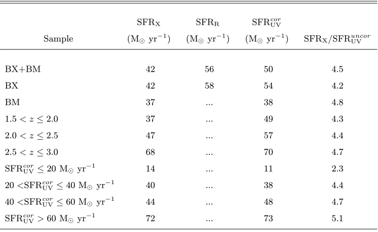
Table 2.2. Star Formation Rate Estimates

SFRX SFRR SFRcorUV

Sample (M⊙ yr−1₎ _(M⊙_yr−1₎ _(M⊙_yr−1₎ _SFR

X/SFRuncorUV

BX+BM 42 56 50 4.5

BX 42 58 54 4.2

BM 37 ... 38 4.8

1.5< z≤2.0 37 ... 49 4.3 2.0< z≤2.5 47 ... 57 4.4 2.5< z≤3.0 68 ... 70 4.7 SFRcor

UV≤20 M⊙yr

−1 ₁₄ _... ₁₁ _2.3

20<SFRcor

UV≤40 M⊙yr

−1 ₄₀ _... ₃₈ _4.4

40<SFRcor

UV≤60 M⊙yr−1 44 ... 48 4.7

SFRcor

UV>60 M⊙yr

(35)

Chapter 3

A Census of Optical and Near-Infrared Selected

Star-Forming and Passively Evolving Galaxies at

Redshift

z

∼

2

∗†

Naveen A. Reddy,a Dawn K. Erb,b Charles C. Steidel,a Alice E. Shapley,c

Kurt L. Adelberger,d & Max Pettinie

a_{California Institute of Technology, MS 105–24, Pasadena, CA 91125}

b_{Harvard-Smithsonian Center for Astrophysics, 60 Garden Street, Cambridge, MA 02138}

c_{Astronomy Department, University of California, Berkeley, 601 Campbell Hall, Berkeley, CA 94720}

d_{McKinsey & Company, 1420 Fifth Avenue, Suite 3100, Seattle, WA 98101}

e_{Institute of Astronomy, Madingley Road, Cambridge CB3 OHA, UK}

Abstract

Using the extensive multi-wavelength data in the GOODS-North field, including our

ground-based rest-frame UV spectroscopy and near-IR imaging, we construct and draw comparisons

between samples of optical and near-IR selected star-forming and passively evolving galaxies

∗_{Based, in part, on data obtained at the W. M. Keck Observatory, which is operated as a scientific}

partnership among the California Institute of Technology, the University of California, and NASA, and was

made possible by the generous financial support of the W. M. Keck Foundation.

(36)

22

at redshifts 1.4_∼< z_∼<2.6. We find overlap at the 70₋80% level in samples of z_∼2 star-forming galaxies selected by their optical (UnGR) and near-IR (BzK) colors when subjected

to commonK-band limits. DeepChandradata indicate a_∼25% AGN fraction among near-IR selected objects, much of which occurs among near-near-IR bright objects (Ks <20; Vega).

Using X-rays as a proxy for bolometric star formation rate (SFR) and stacking the X-ray

emission for the remaining (non-AGN) galaxies, we find the SFR distributions of UnGR,

BzK, and J₋Ks >2.3 galaxies (i.e., Distant Red Galaxies; DRGs) are very similar as a

function of Ks, with Ks < 20 galaxies having hSF Ri ∼ 120 M⊙ yr −₁

, a factor of 2 to 3

higher than those with Ks >20.5. The absence of X-ray emission from the reddest DRGs

and BzK galaxies with (z₋K)AB _∼>3 indicates they must have declining star formation

histories to explain their red colors and low SFRs. While theM/Lratio of passively-evolving galaxies may be larger on average, theSpitzer/IRAC data indicate that their inferred stellar

masses do not exceed the range spanned by optically selected galaxies, suggesting that the

disparity in current SFR may not indicate a fundamental difference between optical and

near-IR selected massive galaxies (M∗

>1011M⊙). We consider the contribution of optical,

near-IR, and submillimeter-selected galaxies to the star formation rate density (SFRD) at

z_∼2, taking into account sample overlap. The SFRD in the interval 1.4_∼< z_∼<2.6 ofUnGR

and BzK galaxies to Ks = 22, and DRGs to Ks = 21 is ∼0.10±0.02 M⊙ yr

−1 _Mpc−3_.

Optically-selected galaxies to _R = 25.5 and Ks = 22.0 account for ∼ 70% of this total.

Greater than 80% of radio-selected submillimeter galaxies toS850µm∼4 mJy with redshifts

1.4< z <2.6 satisfy either one or more of the BX/BM, BzK, and DRG criteria.

3.1

Introduction

A number of surveys have been developed to select galaxies atz_∼2, determine their bolo-metric star formation rates (SFRs), and compare with other multi-wavelength studies to

form a census of the total star formation rate density (SFRD) at z_∼2 (e.g., Steidel et al. 2004; Rubin et al. 2004; Daddi et al. 2004b). A parallel line of study has been to compare

optical and near-IR selected galaxies that are the plausible progenitors of the local

popula-tion of passively evolving massive galaxies. However, biases inherent in surveys that select

galaxies based on their star formation activity (e.g., Steidel et al. 2004) and stellar mass

(37)

with an accurate knowledge of the overlap between these samples can we begin to address

the associations between galaxies selected in different ways, their mutual contribution to

the SFRD at z _∼ 2, and the prevalence and properties of passively evolving and massive galaxies at high redshift. Quantifying this overlap between optical and near-IR surveys is

a primary goal of this paper.

In practice, optical surveys are designed to efficiently select galaxies with a specific

range of properties. The imaging required for optical selection is generally a small fraction

of the time required for near-IR imaging, and can cover much larger areas within that

time. In contrast, near-IR surveys sample galaxies over a wider baseline in wavelength than

optical surveys, and can include galaxies relevant to studying both the star formation rate

and stellar mass densities at high redshift. However, in order to achieve a depth similar

(and area comparable) to that of optical surveys, near-IR selection requires extremely deep

imaging and can be quite expensive in terms of telescope time due to the relatively small size

of IR arrays compared to CCDs. Furthermore, the “color” of the terrestrial background for

imaging is (B₋Ks)AB≃7 magnitudes, much redder than all but the most extremez∼2

galaxies. Once selected, of course, such extreme galaxies then require heroic efforts to obtain

spectra, whereas optical selection, particularly at redshifts where key features fall shortward

of the bright OH emission “forest,” virtually guarantees that one can obtain a spectroscopic

redshift with a modest investment of 8 - 10m telescope time and a spectrograph with

reasonably high throughput. As we show below, optical and near-IR surveys complement

each other in a way that is necessary for obtaining a reasonably complete census of galaxies

at high redshift.

The SFRs of z _∼ 2 galaxies are typically estimated by employing locally calibrated relations between emission at which the galaxies can be easily detected (e.g., UV, Hα) and their FIR emission. The X-ray luminosity of local non-active galaxies results primarily

from high mass X-ray binaries, supernovae, and diffuse hot gas (e.g., Grimm et al. 2002;

Strickland et al. 2004); all of these sources of X-ray emission are related to the star formation

activity on timescales of_∼<100 Myr. Observations of galaxies in the local Universe show a tight correlation between X-ray and FIR luminosity, prompting the use of X-ray emission as

an SFR indicator (Ranalli et al. 2003). This correlation between X-ray emission and SFR

applies to galaxies with a very large range in SFRs, from_∼0.1₋1000 M⊙ yr −₁

(38)

24

analyses at X-ray and radio wavelengths, and comparison with UV emission, indicate that

the local SFR relations appear to give comparable estimates of the instantaneous SFRs

of galaxies after assuming continuous star formation models and correcting for dust (e.g.,

Reddy & Steidel 2004; Nandra et al. 2002; Seibert et al. 2002).

Two surveys designed to select massive galaxies at redshifts 1.4_∼< z_∼<2.5 and passively-evolving (PE) galaxies at redshifts z _∼> 2, respectively, are the K20 and FIRES surveys. The K20 and FIRES selection criteria were developed to take advantage of the sensitivity

of rest-frame optical light and color to stellar mass and the strength of the Balmer break,

respectively, for z_∼2 galaxies (e.g., Cimatti et al. 2002a; Franx et al. 2003). The Gemini Deep Deep Survey (GDDS) extends this near-IR technique to target massive galaxies at

slightly lower redshifts (0.8_∼< z_∼<2.0; Abraham et al. 2004).

X-ray stacking analyses of the brightest galaxies in the K20 and FIRES surveys indicate

an average SFR a factor of 4 to 5 times larger than for optically-selected z _∼ 2 galaxies (Daddi et al. 2004a; Rubin et al. 2004), inviting the conclusion that optical selection misses

a large fraction of the star formation density at high redshift. While it is certainly true

that optical surveys miss some fraction of the SFRD, the past quoted difference in the

average SFRs of galaxies selected optically and in the near-IR disappears once the galaxies

are subjected to a common near-IR magnitude limit, as we show below.

We have recently concluded a campaign to obtain deep near-IR imaging for fields in the

z _∼ 2 optical survey (Steidel et al. 2004), allowing for a direct comparison of optical and near-IR selected galaxies. One result of this comparison is that Ks <20 (Vega)

optically-selected galaxies show similar space densities, stellar masses, and metallicities as Ks-bright

galaxies in near-IR samples (Shapley et al. 2004). More recently, Adelberger et al. (2005a)

show that the correlation lengths forKs-bright galaxies among optical and near-IR samples

are similar, suggesting an overlap between the two sets of galaxies, both of which plausibly

host the progenitors of massive elliptical galaxies in the local Universe. These results suggest

that near-IR bright galaxies have similar properties regardless of the method used to select

them.

In this paper, we extend these results by examining the color distributions and

(39)

complementary data available, includingChandra/X-ray, ground-based optical and near-IR,

and Spitzer/IRAC imaging. Multi-wavelength data in a single field are particularly useful

in that we can use a common method for extracting photometry that is not subject to the

biases that may exist when comparing galaxies in different fields whose fluxes are derived

in different ways. The addition of our rest-frame UV spectroscopic data in the

GOODS-N field provides for a more detailed analysis than otherwise possible of the properties of

galaxies as a function of selection technique. Furthermore, the GOODS-N field coincides

with the ChandraDeep Field North (CDF-N) region which have the deepest (2 Ms) X-ray

data available (Alexander et al. 2003). The X-ray data allow for an independent estimate

of bolometric SFRs and the available depth allows more leeway in stacking smaller numbers

of sources to obtain a statistical detection, as well as identifying AGN to a lower luminosity

threshold than possible in other fields that have shallower X-ray data.

The outline of the paper is as follows. In _§ 2, we describe the optical, near-IR, X-ray,

and IRAC data and present the optical and near-IR selection criteria and X-ray stacking

method. Color distributions, direct X-ray detections, and stacked results are examined in

§ 3. In_§ 4, we discuss the SFR distributions of optical and near-IR selectedz_∼2 galaxies and their relative contributions to the SFRD, and the presence of a passively evolving

population of galaxies. A flat ΛCDM cosmology is assumed with H0 = 70 km s−1 Mpc−1

and ΩΛ= 0.7.

3.2

Data and Sample Selection

3.2.1 Imaging

Optical UnGR images in the GOODS-North field were obtained in April 2002 and 2003

under photometric conditions using the KPNO and Keck I telescopes. The KPNO/MOSAIC

U-band image was obtained from the GOODS team (PI: Giavalisco) and was transformed to reflect Un magnitudes (e.g., Steidel et al. 2004). The Keck IG andRband images were

taken by us with the Low Resolution Imaging Spectrograph (LRIS; Oke et al. 1995, Steidel

et al. 2004), and were oriented to provide the maximum overlap with the GOODS ACS and

Spitzersurvey region. The images cover 11′ ×15′

with FWHM_∼0′′.

(40)

26

Steidel et al. (2003). We obtained deepB-band images of the GOODS-N field from a public distribution ofSubaru data (Capak et al. 2004). The deep z-band data are acquired from the public distribution of the HST Advanced Camera for Surveys (ACS) data (Giavalisco et al. 2004b). The B and z band data have 5 σ depths of 26.9 and 27.4 mag measured in 3′′

and 0′′.

2 diameter apertures, respectively. TheKs andJ imaging was accomplished with

the Wide Field Infrared Camera (WIRC) on the Palomar Hale 5 m telescope (Wilson et al.

2003), providing 8.′

7 _× 8.′

7 coverage in the central portion of the GOODS-N field. The

near-IR images cover _∼ 43% of the optical image. The images had FWHM _∼ 1′′.

0 under

photometric conditions and 3 σ sensitivity limits of _∼22.6 and_∼24.1 mag in theKs and

J bands, respectively. The near-IR data are described in detail by Erb et al. (2006c). The total area studied in the subsequent analysis is_∼72.3 arcmin2.

The procedures for source detection and photometry are described in Steidel et al.

(2003). Briefly,UnGR magnitudes were calculated assuming isophotal apertures that were

adjusted to the_R-band flux profiles. Source detection was done at Ks-band. BzK and J

magnitudes are computed assuming the isophotal apertures adjusted to the Ks-band flux

profiles, unless the_R-band isophotes gave a more significantKsdetection. In the analysis to

follow, “Ks” andJ magnitudes are in Vega units. We use the conversionKAB=Ks+ 1.82.

All other magnitudes are in AB units.

Fully reducedSpitzer/IRAC mosaics of the GOODS-North field were made public in the

first data release of the GOODS Legacy project (PI: Dickinson). The IRAC data overlap

completely with our Ks-band image, but currently only two channels (either 3.6 µm and

5.8µm, or 4.5µm and 8.0µm) are available over most of the image. A small area of overlap has coverage in all four channels. The images are deep enough that source confusion is an

issue. We have mitigated the effects of confusion noise by employing the higher spatial

resolutionKs-band data to constrain source positions and de-blend confused IRAC sources.

We performed PSF photometry using the procedure described in Shapley et al. (2005).

3.2.2 Selection Criteria

3.2.2.1 Optical Selection of Star-Forming Galaxies

We have optically-selected z _∼ 2 galaxies in the GOODS-N field based on their observed

(41)

25.5. The selection criteria aim to select actively star-forming galaxies at z _∼ 2 with the same range in UV properties and extinction as LBGs at z_∼3 (Steidel et al. 2003). “BX” galaxies are selected to be at redshifts 2.0_∼< z_∼<2.6 using the following criteria:

G_{− R ≥ −}0.2

Un−G ≥ G− R+ 0.2

G_{− R ≤} 0.2(Un−G) + 0.4

Un−G ≤ G− R+ 1.0, (3.1)

and “BM” objects are selected to be at redshifts 1.5_∼< z_∼<2.0 using the following criteria:

G_{− R ≥ −}0.2

Un−G ≥ G− R −0.1

G_{− R ≤} 0.2(Un−G) + 0.4

Un−G ≤ G− R+ 0.2 (3.2)

(Adelberger et al. 2004; Steidel et al. 2004). For subsequent analysis, we will refer to BX

and BM objects as those that are optically-, or “BX/BM”-, selected. Optical color selection ofz_∼2 galaxies in the 11′

by 15′

area of the GOODS-North field

yielded 1360 BX and BM candidates, of which 620 lie in the region where we have

comple-mentary J₋ and K-band data (_§ 3.2.1), and 199 have Ks < 21.0. Followup spectroscopy

with the blue channel of the Low Resolution Imaging Spectrograph (LRIS-B) yielded 147

redshifts for objects with Ks-band data (248 redshifts over the entire optical field). Of

these 147 objects with redshifts andKs-band data, 129 have z >1, and 60 havez >1 and

Ks <21. The mean redshift of the 60 BX/BM objects is hzi= 1.99±0.36. The

spectro-scopic interloper fractions in the BX/BM sample are summarized in Table 3.1. The BX and BM selection functions (shown as shaded distributions in Figure 3.1) have distributions

(42)

28

Figure 3.1Spectroscopicredshift distributions toKs = 21 for the various samples considered

here. The BX/BM and BzK/SF distributions (hashed histograms) include sources from our sample in the GOODS-North field and overlap almost completely. The DRGs have a

higher mean redshift of_hz_i= 2.48_±0.38 from our sample ofJ₋Ks >2.3 sources withz >1

in all four fields of the optical survey (Steidel et al. 2004) where we have complementaryJ₋

andK-band imaging. The redshift distribution of DRGs within our sample (all of which are selected with the BX/BM or z_∼3 LBG criteria) is similar to that found by van Dokkum et al. (2004), van Dokkum et al. (2003), and F¨orster Schreiber et al. (2004b). The solid

histogram shows the redshift distribution for BzK/PE galaxies from Daddi et al. (2004a) and Daddi et al. (2005b), scaled down by a factor of 3 for clarity. The background shaded

regions show the arbitrarily normalized redshift distributions for optically-selected BX and

(43)

3.2.2.2 Near-IR Selection of Star-Forming Galaxies

The near-IR properties of galaxies can be used both to target star forming galaxies and to

identify those with extremely red colors that may indicate passive evolution. To address the

former issue, we have employed the “BzK” selection criteria of Daddi et al. (2004a) to cull objects in the GOODS-N field and directly compare with those selected on the observed

optical properties ofz_∼>2 galaxies. Daddi et al. (2004a) define the quantity “BzK”:

BzK _≡(z₋K)₋(B₋z); (3.3)

star-forming galaxies withz >1.4 are targeted by the following criterion:

BzK _{≥ −}0.2, (3.4)

in AB magnitudes. Of the 1185 sources with>3σ B,z, andKdetections andKs <21, 221

satisfy Equation 3.4. The surface density of BzK galaxies with Ks <21 is ∼3 arcmin−2,

similar to the surface density of BX/BM galaxies to a similar Ks-band depth. These

star-forming BzK galaxies will be referred to as “BzK/SF” galaxies, and their spectroscopic redshift distributionfrom our spectroscopic sampleis shown in Figure 3.1. Our deep near-IR

imaging allows us to determine the redshift distribution forBzK/SF galaxies withKs>20

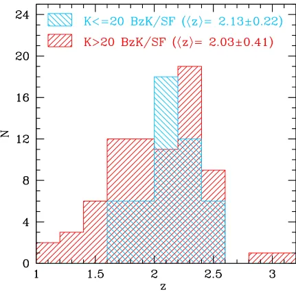
(and which also satisfy the BX/BM criteria), and the results are shown in Figure 3.2. The mean redshifts of the Ks ≤ 20 and Ks > 20 distributions are hzi = 2.13±0.22 and hz_i = 2.03_±0.41, respectively, and agree within the uncertainty. We note, however, that theBzK/SF criteria selectKs >20 objects over a broader range in redshift (1.0≤z≤3.2)

than Ks ≤20 objects. This reflects the larger range in BzK colors of Ks > 20 BzK/SF

galaxies compared with those having Ks ≤ 20. Additionally, the photometric scatter in

colors is expected to increase for fainter objects, so a broadening of the redshift distribution

forBzK/SF objects with fainterKs magnitudes is not surprising.

We emphasize that we only know the redshifts for BzK/SF galaxies that also happen to fall in the BX/BM sample. In general, the true redshift distribution,NoBzK/SF(z), of the

(44)

30

Figure 3.2 Arbitrarily normaliz