Cryptosystem
Taylor Daniels1 and Daniel Smith-Tone1,2 1Department of Mathematics, University of Louisville,
Louisville, Kentucky, USA
2National Institute of Standards and Technology, Gaithersburg, Maryland, USA
[email protected],[email protected]
Abstract. Multivariate Public Key Cryptography (MPKC) has been put forth as a possible post-quantum family of cryptographic schemes. These schemes lack provable security in the reduction theoretic sense, and so their security against yet undiscovered attacks remains uncertain. The effectiveness of differential attacks on various field-based systems has prompted the investigation of differential properties of multivariate schemes to determine the extent to which they are secure from differ-ential adversaries. Due to its role as a basis for both encryption and signature schemes we contribute to this investigation focusing on the
HF E cryptosystem. We derive the differential symmetric and invariant structure of theHF E central map and that ofHF E− and provide a collection of parameter sets which make theseHF E systems provably secure against a differential symmetric or differential invariant attack.
1
Introduction and Outline
Along with the discovery of polytime quantum algorithms for factoring and com-puting discrete logarithms, see [1], came a rising interest in “quantum-resistant” cryptographic protocols. For the last two decades this interest has blossomed into a large international effort to develop post-quantum cryptography, a term which elicits visions of a post-apocalyptic world where quantum computing ma-chines reign supreme. While progress in quantum computing indicates that such devices are not precluded by the laws of physics, it is not at all clear when we may see large-scale quantum computing devices becoming a cryptographic threat. Nevertheless, the potential and the uncertainty of the situation clearly establish the need for secure post-quantum options.
While it is difficult to be assured of a cryptosystems’s post-quantum secu-rity in light of the continual evolution of the relatively young field of quantum algorithms, it is reasonable to start by developing schemes which resist classical attack and for which there is no known significant weakness in the quantum realm. Furthermore, the establishment of security metrics provide insight which educate us about the possibilities for attacks and the correct strategies for the development of cryptosystems.
In this vein, some classification metrics are introduced in [2, 3] which can be utilized to rule out certain classes of attacks. While not reduction theoretic attacks, reducing the task of breaking the scheme to a known (or often suspected) hard problem, these metrics can be used to prove that certain classes of attacks fail or to illustrate specific computational challenges which an adversary must face to effect an attack.
Many attacks on multivariate public key cryptosystems can be viewed as differential attacks, in that they utilize some symmetric relation or some invari-ant property of the public polynomials. These attacks have proved effective in application to several cryptosystems. For instance, the attack on SFLASH, see [4], is an attack utilizing differential symmetry, the attack of Kipnis and Shamir [5] on the oil-and-vinegar scheme is actually an attack exploiting a differential invariant, even Patarin’s initial attack on C∗ [6] can be viewed as an exploita-tion of a trivial differential symmetry, see [3]. These attacks are evidence that the work in [2, 3] is worthy of continuation and further development.
This task leads us to an investigation of the HF E family of schemes, see [7], and a characterization of the differential properties of some variants. Results similar to those of [2, 3] will allow us to make conclusions about the differential security ofHF E-derived schemes, and, in particular, provide some insight into the properties of some of its important variants such as HF E− and HF Ev−, see [8] and [9].
To this end, we derive the differential symmetry and differential invariant structure of the central map of HF E. Specifically, we are able to bound the probability that anHF E primitive has a nontrivial differential structure and to provide parameter sets for which HF E is provably secure against a differential adversary. This result on the HFE primitive, in conjunction with degree of reg-ularity results such as [10, 11] provide a strong argument for the security of the
HF E− andHF Ev− signature schemes, though more work is required to verify that the differential structure is not weakened by the minus or vinegar modifiers for practical parameters.
differen-tial invariant in the general case. Finally, we conclude, noting parameters which provide provable differential security.
2
The Differential Adversary
The discrete differential of a field map f :Fnq →Fmq is given by:
Df(y, x) =f(x+y)−f(x)−f(y) +f(0).
It is simply a normalized difference equation with variable interval. Several prominent cryptanalyses in the history of MPKC have utilized a symmetric relation of the discrete differential of the core map or subspaces which are left invariant under some action of the differential of the core map. Simple exam-ples include the linearization equations attack of [7], which can be viewed as exploiting the relationDf(f(x), f(x)) = 0; the attack on balanced Oil-Vinegar, see [12, 5]; and the SFLASH attack of [4]. Along with rank attacks, differential attacks have made the greatest impact on MPKC among structural key recovery attacks.
For the purpose of progress in security analysis in MPKC, we propose a model for a differential adversary. This model strives to capture the behaviors employed in all differential attacks and will hopefully be improved with time.
We will say that adifferential adversary A, is a probabilistic Turing machine with access to a public keyP which computes either
1. an affine mapL such thatDP(Ly, x) +DP(y, Lx) =ΛLDP(y, x), or 2. a pair of subspacesV W withdim(V)+dim(W)≥nthe number of variables,
such thatDP(y, x) = 0 for allx∈V andy∈W,
and uses the solution to derive an equivalent private key.
We note specifically that it suffices to prove that a core mapf has no such
L and no such (V, W) to guarantee that the differential adversary’s advantage for the cryptosystem with primitivef is zero. Item 1 above is discussed in more detail in Section 4 and item 2 in Section 5.
3
HFE
The Hidden Field Equations (HF E) scheme was first presented by Patarin in [7] as a method of avoiding his linearization equations attack on the C∗ scheme of Matsumoto and Imai, see [6] and [13]. The basic idea of the system is to use the butterfly construction to hide an easily invertible polynomial over an extension field.
composition over the base field, Fq. Explicitly any such “core” map f has the form:
f(x) = X i≤j qi+qj<D
αi,jxq
i+qj
+ X
i qi<D
βixq
i
+γ,
with the degree bound Destablished to allow for easy inversion.
To encrypt given the public key P(x), one simply evaluates every public polynomial at the plaintext vectorx∈Fnq ≈K. Decryption is accomplished by inverting each of the three private components individually. The most interesting inversion is that of f, which is inverted via a polynomial system solver such as the Berlekamp algorithm.
In [7], Patarin presented a couple ofHF E challenges to be used as bench-marks for progress in cryptanalyzingHF E andHF E−.HF E challenge 1 was broken in 2003, see [14], via an algebraic attack which allows the direct inversion of the system of equations. This attack was specialized in the sense that it took advantage of the choices of the coefficients off as well as the characteristic of
Fq.
In 2011, HF E was broken altogether in [15], in a vast improvement of the Kipnis-Shamir attack of [16]. The attack breaks the originalHF Efor all practi-cal parameters as well as several variants, including projectedHF E and
Multi-HF E, by what amounts to a sophisticated rank analysis of the central map via the public polynomials. Notably, the attack cannot break HF E− orHF Ev−.
4
Linear Differential Symmetry
4.1 Symmetry for HFE
In [4], the SFLASH signature scheme was broken by exploiting a symmetric relation of the differential of the public key. This relation was inherited from the core map of the scheme. Specifically, a linear differential symmetry is an equation in which linear maps are applied to the differential in such a way that the equation is linear in the unknown coefficients of the linear maps. We can always express the symmetry in the following form:
Df(M y, x) +Df(y, M x) =ΛMDf(y, x), (1)
where M and ΛM are linear maps. To evaluate the potential for a differential symmetric attack onHF E, we consider conditions for the existence of a linear differential symmetry on the core mapf of anHF E scheme.
Consider the differential of the core map:
Df(y, x) = X i≤j qi+qj<D
Df is aK-bilinear form. We choose a convenient representation forK:
x7→
x xq
.. .
xqn−1
.
Under this representation we can express Df as the n×n symmetric matrix with (i, j)th and (j, i)th entriesαi,jfori6=jand (i, i)th entry 2αi,i(which may be zero depending on the characteristic ofK).
Since any linear mapM :K→Kcan be writtenM x=Pn−1 i=0 mixq
i
, under our representationM can be expressed:
M =
m0 m1 . . . mn−1
mqn−1 mq0 . . . mqn−2
..
. ... . .. ...
m1qn−1m2qn−1 . . . mq0n−1
.
In this representation, we have the formula
Df(M y, x) +Df(y, M x) =y(MTDf+Df M)x. (3)
Consider the action ofΛM onDf.ΛMDf(y, x) =P n−1
k=0λkDf(y, x)q
k
. Notice specifically that in our representation the matrix for Dfqk
is the same as the matrix representing Df shifted to the right and down k units with all entries raised to theqkth power. This shift is due to the fact that
Df(y, x)qk= X i≤j qi+qj<D
αqi,jk(yqi+kxqj+k+yqj+kxqi+k).
Specifically, the (i, j)th entry of Dfqk is αqk
i−k,j−k if i 6= j, and (i, i)th entry (2αi−k,i−k)q
k
= 2αqi−kk,i−k (0 in characteristic two).
Thus the possibility of a differential symmetry can be deduced simply by setting the matrix MTDf +Df M equal to the matrix Λ
MDf. With certain constraints it is easy to deduce whether there exists a solution.
Theorem 1 Letf(x)be anHF E polynomial (in particularf is not a monomial function). Suppose thatf has the following properties:
1. no power ofq is repeated among the exponents off, and 2. the difference of the powers ofqin each exponent is unique.
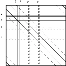
s i i j j r r s
Fig. 1.Graphical representation of the equationMTDf+Df M =Λ
MDffor theHF E
polynomial f(x) = αi,jxq
i+qj
+αr,sxq
r+qs
. Horizontal and vertical lines represent nonzero entries in MTDf +Df M while diagonal lines represent nonzero entries in ΛMDf. Solid lines correspond to the (i, j) monomial while dotted lines correspond to
the (r, s) monomial.
Proof. First consider computing Df M. From the condition on the monomials of f, Df has at most a single nonzero entry in any row or column. Therefore each row of Df M is a multiple of a row in M. In particular, if αi,jxq
i+qj
is a monomial off, then theith row ofDf M is
h
αi,jmq
j
−j αi,jmq
j
1−j. . . αi,jmq
j
−1−j i
,
and thejth row is
h
αi,jm qi
−iαi,jm qi
1−i. . . αi,jm qi
−1−i i
.
Consider theith row ofMTDf+Df M. For allknot occurring as a power ofqin
f, the (i, k)th entry isαi,jmq
j
k−j. Consider the (i, j)th entry ofM
TDf+Df M. This quantity is the sum of the (i, j)th entry of Df M and the (j, i)th entry,
specificallyαi,j(mq0i+mq0j). Letαr,sxq
r+qs
be another monomial off. Then the
(i, r)th entry ofMTDf+Df M isα i,jm
qj
r−j+αr,sm qs
i−s, and the (i, s)th entry is
αi,jmq
j
s−j+αr,smq
r
i−r. InΛMDf, for all αi,jxq
i+qj
a monomial in f, the (i+k, j+k)th entry is
equal to the (j +k, i+k)th entry and takes the value αqi,jkλk while all other entries are zero.
Therefore consider the elements in the ith row of the equation MTDf +
Df M =ΛMDf. For every monomialαr,sxq
r+qs
inf, we have that thes−r+ith element and ther−s+ith element of row i in ΛMDf are nonzero. All other entries of that row are zero. Therefore, for all k not occurring as a power of q
plusi,mk−j = 0. Given the condition that the differences of powers ofq in the exponents are unique, and the equations mk−t= 0 for all other t occurring as powers ofq, we obtainmi= 0 for alli6= 0. ThereforeM is a multiplication map. But as proven in Theorem 2 in [17], ifm06∈Fq this implies that the polynomial is a C∗ monomial, a contradiction. Thus M is simply multiplying by a scalar which induces a symmetry for every map g:K→K. Thusf has no nontrivial differential symmetry.
4.2 Symmetry for HF E−
We can extend the result of the previous section to reveal the differential sym-metric structure ofHF E−. The specific difference in the proof is merely placing the operatorπ, a projection on to a subspace, in (3).
π
MTDf+Df M
=ΛM[Df]. (4)
We handle the case of a codimension 1 projection explicitly. The following argument can be easily generalized to a codimensionrprojection.
Theorem 2 Let Kbe a prime extension ofFq and letπ:K→Kbe a codimen-sion1 projection. Suppose thatf has the following properties:
1. no power ofq is repeated among the exponents off,
2. the difference of the powers ofqin each exponent is unique,
3. the difference between any two powers of q among the exponents is at least two, and
4. there exist two monomialsαi,jxq
i+qj
andαqr+qs
r,x such thatα
(q−1)(q1−i−q1−j+qj−qi)
q2i−2j−1
i,j 6=
α
(q−1)(q1−r−q1−s+qs−qr)
q2r−2s−1
r,s .
Then ifD(π◦f)(M y, x) +D(π◦f)(y, M x) =ΛMDf(y, x), thenM x=m0xfor somem0∈Fq. Thus π◦f has no nontrivial differential symmetry.
Proof. Due to the effect of T, we may without loss of generality assume that
πx =x+xq. Therefore, the matrix form of πMTDf+Df M is the sum of the matrix form of MTDf+Df M and itself with every element raised to the powerqand transposed one row down and one row to the right.
Following the argument of Theorem 1 reveals thatmi= 0 for alli6=−1,0,1. For each monomialαi,jxq
i+qj
inf, we obtain the relations
αi,jmq
j
1 +α q i,jm
qi+1 −1 = 0
αi,jmq
i
1 +α q i,jm
qj+1 −1 = 0,
(5)
s i
i
r
r
j
j s
Fig. 2.Graphical representation of the equationπ
MTDf+Df M
=ΛMDf for the HF E polynomial f(x) = αi,jxq
i+qj
+αr,sxq
r+qs
, where πx = x+xq. Horizontal
and vertical lines represent nonzero entries inπ
MTDf+Df M
while diagonal lines represent nonzero entries inΛMDf. Solid lines correspond to the (i, j) monomial while
dotted lines correspond to the (r, s) monomial.
Given condition (4), there exist two monomials with independent solution sets, thusm−1=m1= 0.
Finally, collecting equations involvingm0we obtain for each monomial:
αi,jm qj
0 +αi,jm qi
0 =αi,jλ0
αqi,jmq0j+1+αqi,jmq0i+1=αqi,jλ1.
(6)
Since M x=m0x, we may apply Theorem 2 from [17] in the casem0 6∈Fq to conclude thatπ◦f is a quadratic monomial map. This fact contradicts condition (3), however, and thusm0∈Fq.
We note that the conditions of the above theorem are very easy to check, though for very small D they may be difficult to satisfy and there may be some issues regarding a lack of entropy in the private key space. With proper selection of the extension, however, it is unlikely that this adjustment will lead to a successful attack based on the morphism of polynomials problem, in a similar vein to [18].
5
Differential Invariants
5.1 Definitions and Implications
The discrete differential Df is a symmetric, bilinearfunction onFnq (using the vector space representation of K), but each coordinate of Df is a symmetric, bilinear form on K. Because of this, we may express each coordinate of Df, [Df(y, x)]i as
Maintaining our definitions ofKand f, we define a “first order differential invariant” off.
Definition 1 Let f : K → K be a function. A differential invariant of f is a subspace V ⊆ K with the property that there is a subspace W ⊆ K such that
dim(W)≤dim(V)and∀A∈SpanFq(Dfi),AV ⊆W.
Informally speaking, a function has a differential invariant if the image of a sub-space under all differential coordinate forms lies in a fixed subsub-space of dimension no larger. This definition captures the notion of simultaneous invariants, sub-spaces which are simultaneously invariant subsub-spaces ofDfi for alli, and detects when large subspaces are acted upon linearly.
If we assume the existence of a first order differential invariant V, we can define a corresponding subspace V⊥ as the set of all elements x∈
Ksuch that the dot product hx, Avi = 0 ∀v ∈ V,∀A ∈ Span(Dfi). This is not quite the usual definition of an orthogonal complement. V⊥ is not the set of everything orthogonal to V, but rather everything orthogonal to AV, which may or may not be inV.
With our definitions of V and V⊥, we can establish the following useful result. Assume there is a first order differential invariant V ⊆ K, and pick a linear projection M : K → V and another linear projection M⊥ :
K → V⊥. Examining one of the differential coordinate-forms,
[Df(M⊥y, M x)]i= (M⊥y)T(Dfi(M x)) (7)
SinceM⊥y is in V⊥, andDfiM x∈AV, we must then have that
[Df(M⊥y, M x)]i= (M⊥a)T(Dfi(M x)) = 0 (8)
The “i” inDfi did not matter, meaning that for alli (from 1 ton), i.e. for all coordinates of Df, the above equation is true. We can then simply say that:
∀y, x∈K, Df(M⊥y, M x) = 0 or equivalently, Df(M⊥K, MK) = 0 (9)
This fact will restrict whatM andM⊥ can be.
5.2 M⊥=SM T
We can make our investigation ofM, M⊥easier by employing a small result from linear algebra. Our idea is to express M⊥ = SM T, where S may be singular, butT is nonsingular (or vice versa ifrank(M)< rank(M⊥)). The result we use is:
Proof. LetAbe anm×nmatrix of rankr. With row operations (P, m×m) we can getAinto row echelon form,P A. Then we can use column operations (Q, n×n) to “zero-out” the remaining nonleading elements and permute the leading 1’s to the first rcolumns. Thus P AQis the m×n matrix with ther×r identity matrix in the upper-left region, and zeros everywhere else. Denote this matrix asI0. ThusP AQ=I0. We can also do this withB, so thatP0BQ0=I0=P AQ. ThusA= (P−1P0)B(Q0Q−1), withP−1P0 andQ0Q−1 nonsingular.
Without loss of generality, due to the symmetry of Df, we may assume that rank(M⊥) ≤ rank(M). If the ranks are equal, then we may apply the proposition and writeM⊥ =SM T, withS andT nonsingular. Ifrank(M⊥)< rank(M), composeM with a singular matrixXso thatrank(XM) =rank(M⊥), and then apply the result so that M⊥ = S(XM)T. Then we can express
M⊥ = S0M T, where S0 is singular. The matrix T is included to ensure that the kernels of M, M⊥ are properly aligned. Restating our differential result (9) in this manner, we have that ifM⊥=SM T, andM :K→V, then
∀x, y∈K, Df(SM T y, M T x) = 0 (10)
5.3 Minimal Polynomial
Definition 1. We define the minimal polynomial of a subspaceV ⊆Kas
MV(x) = Y
v∈V (x−v)
The term “minimal polynomial” is used since this is the polynomial of minimal degree of which every element ofV is a root. We note that the equationMV(x) = 0 is anFq-linear equation.
Suppose that V has Fq-dimension d, so that |V| = qd. Then MV(x) has degreeqd and, in keeping with our previous descriptions, must have form
xqd+bd−1xq
d−1
+· · ·+b2xq 2
+b1xq+b0x bi ∈K (11) More generally, we can characterize all functions fromV to K:
Proposition 2. Let FV be the ring of all functions from the Fq-subspace V of KtoK. ThenFV is isomorphic to K[x]/hMV(x)i.
Proof. The ring of all functions from K to itself is K[x]/xq
n
−x
. Suppose that f, g ∈K[x]/xq
n
−x
are identical on V. Then for all v ∈V, v is a root of (f−g)(x). Thus (x−v) is a linear factor of (f −g)(x) for allv ∈V. Thus
MV(x)|(f−g)(x). Consequently,hMV(x)iis the ideal of functions which send
V to zero. ThusK[x]/xq
n
−x,MV(x)
is the ring of nontrivial functions from
V to K. Since MV(x) splits in K, MV(x)|xq
n
−x. To see that all functions from V to K are polynomials note that there are (qn)q
d
functions from V (of
Fq-dimensiond) toK, and|K[x]/hMV(x)i |= (qn)q
d
6
Differential Invariant Structure
6.1 HFE
If f has non-trivial invariant V we know that ∀A ∈ Span(Dfi), dim(AV) ≤
dim(V). Since the dot-product is non-degenerate onK, and remembering that
V⊥is defined slightly differently, we can saydim(V⊥) +dim(AV) =n. This fact implies thatdim(V⊥)+dim(V)≥n, so eitherdim(V⊥)≥n/2 ordim(V)≥n/2, possibly both.
Ifdim(V)≥n/2, we maintainM T :K→V and characterizeS:V →V⊥. If we deduceS mapsV to {0}, that is,V⊥ ={0}, this would meandim(AV) =n
and consequently AV =K. IfV 6=K, we contradictdim(AV)≤dim(V), and if
V =K, we contradict the non-triviality ofV.
Ifdim(V⊥) ≥n/2, we take M0T0 : K→ V⊥ instead and characterize S0 :
V⊥→V. IfS0 is the zero map onV⊥, i.e.S0V⊥=V ={0}, then we contradict the non-triviality ofV.
Without loss of generality we assume dim(V)≥n/2 because the following analysis and results can be achieved just as easily if we havedim(V⊥)≥n/2.
For notational convenience, we now fixM T x= ˆx,M T y= ˆy, andM TK=V. Starting with the core map
f(x) = X i≤j qi+qj<D
αi,jxq
i+qj
+ X
i qi<D
βixq
i
+γ,
we compute:
Df(Sy,ˆ xˆ) = X i≤j qi+qj<D
αi,j h
(Syˆ)qixˆqj+ (Syˆ)qjxˆqii. (12)
For practical parameters, D is far smaller than |V|, see for example [7], and so forDf(Sy,ˆ xˆ) = 0, every coefficient of ˆxqj must be inhMV(ˆy)i. Expanding (12) we obtain:
Df(Sy,ˆ ˆx) = X i≤j qi+qj<D
αi,j h
(Syˆ)qixˆqj+ (Syˆ)qjxˆqii
= X
i,j qi+qj<D
h
(αi,j+αj,i) (Syˆ)q
ii ˆ
xqj,
(13)
where we specifically note in the last expression that ifi6=j exactly one ofαi,j andαj,imay be nonzero. Thus for eachjsuch thatqj< Dwe have the following polynomial:
X
i:qi+qj<D
(αi,j+αj,i)(Syˆ)q
i
The membership of the jth polynomial of the form (14) inhMV(ˆy)i provides the relation
X
i:qi+qj<D
(αi,j+αj,i)(Syˆ)q
i
= 0. (15)
Relation (15) has ` = blogq(D)c degrees of freedom on S as a linear action onV. Therefore, there ared−` Fq-linearly independent relations onS from a single monomial of (13). For a practically chosen D, two linearly independent relations of this form on S force S to be the zero map onV. Consequently, we have thatV⊥={0}, a contradiction. Specifically, the probability that two such given relations are independent is approximately 1−q−n`; thus with very high probability f has no differential invariant structure.
In particular, we provide a specific strategy for provably eliminating differ-ential invariants.
Theorem 3 Letf be anHF E polynomial with degree boundD < qn/2. If there is a power of qwhich is unique, f has no non-trivial invariant structure.
Proof. Assume by way of contradiction thatf has a non-trivial differential in-variant. Let j be the unique power of qoccurring in an exponent in f. By the above discussion it suffices to analyze membership of the jth polynomial of the form (14) in hMV(ˆy)i. Given the condition on j, this polynomial has the form (αrj+αjr)(Syˆ)q
r
. If this polynomial is inhMV(ˆy)i, then so isSyˆ, sinceMV(ˆy) has no repeated factors, and we haveSV ={0}, a contradiction.
6.2 HFE−
Deriving the differential invariant structure forHF E− follows a nearly identical line of reasoning. The clear distinction is that since the definition of the differen-tial invariant depends on the span of the differendifferen-tials of the public polynomials, there is greater freedom to have an invariant when there are fewer public poly-nomials.
Once again, considering the effects of T, it suffices to analyze π◦f where
πx=x+xq. Notice that we have:
π◦f(x) = X i≤j qi+qj<D
αi,jxq
i+qj
+ X i qi<D
βixq
i
+γ
+ X
i≤j qi+qj<D
αqi,jxqi+1+qj+1+ X i qi<D
βiqxqi+1+γq,
(16)
and therefore,
D(π◦f)(Sy,ˆ xˆ) = X i≤j qi+qj<D
αi,j h
(Syˆ)qixˆqj + (Syˆ)qjxˆqii
+ X
i≤j qi+qj<D
αqi,jh(Syˆ)qi+1ˆxqj+1+ (Syˆ)qj+1xˆqi+1i.
Again, we collect terms with respect to the powers of ˆx:
D(π◦f)(Sy,ˆ xˆ) = X
i:qi+1<D
(αi,0+α0,i) (Syˆ)q
i
ˆ
x
+ X
i,(j>0) qi+qj<D
(αi,j+αj,i+αqi−1,j−1+α q
j−1,i−1) (Syˆ) qi
ˆ
xqj
+ X
i,(j>0) qi−1+qj−1<D<qi+qj
(αqi−1,j−1+αqj−1,i−1) (Syˆ)qixˆqj.
(18)
In the last summation, there is a single icorresponding to eachj >0.
Despite the added difficulty of the minus modifier, we can prove the nonexis-tence of nontrivial differential invariants forHF E−under conditions very similar to those provided in the previous subsection.
Theorem 4 Let f be an HF E polynomial with degree bound D < qn/2. Let π
be the codimension 1 projection πx=x+xq. If there is a power ofq which is unique and one less than this power does not occur in any quadratic monomial summand,π◦f has no non-trivial invariant structure.
Proof. By the above condition, there is a power j such that the “coefficient” ofxqj
in (18) comes from exactly one of the summations in (18). Applying the argument from Theorem 3, we have that SV ={0}, and therefore there is no nontrivial differential invariant ofπ◦f.
7
IP, Degree of Regularity, Other Factors
The restrictions suggested in Theorems 1, 2, 3, and 4 reduce the entropy of the private key space, which might raise concerns about vulnerability to attacks based on a “guess-then-IP” strategy, to direct inversion via Gr¨obner bases. As it turns out, for even modest parameters these issues are not realized. Moreover, the theorems are not “tight,” meaning that they are merely simple ways of eliminating differential symmetric and invariant weakness.
Consider, for example, using the parameter set forHF EChallenge 2; specifi-cally, we haveq= 16, n= 36,r= 4, andD= 4352 = 162+ 163. Thus
K=F1636, and ourHF E map must have the form :
f(x) = X i≤j≤3,i6=3
αi,jxq
i+qj
+X i≤3
βixq
i
+γ
may be seen to be equivalent keys (counting equivalence classes of keys inter-sected with polynomials of this form), via the additive and big sustainers of [19]. Therefore, there are roughly q5n nonequivalent polynomials with only α1,2 and
α0,3 nonzero among theα.
For weak parameters, in particular when the αi,j are chosen from the base field, an attack based on the IP problem is presented in [18]. The symmetries used in that method, however, are not present when both α1,2 and α0,3 are chosen randomly from K. While we may consider the coefficient of α1,2 to be “absorbed” by the affine map T, the effect of the remaining coefficient breaks the symmetry. Without the commutativity of the Frobenius map with theHF E
polynomial, the parameters supplied are out of range for an IP-based attack. Another concern is that the rank of the scheme may be so low as to make the scheme susceptible to attack via Gr¨obner basis methods. However, using the theorem from [20], we compute the degree of regularity of the adjusted scheme to be:
(16−1)4
2 + 2 = 32,
based on the fact that the rank of the central map is only four. Using the formula from [21], we obtain an estimated complexity of
36 + 32
32 ω
where ω = 2.3766. Thus, we estimate the complexity of directly inverting this concrete example to beO(2153). Note, the attack of [15] is not feasible here since this is anHF E− scheme, see section 8.1 in [15].
8
Conclusion
For eighteen years, HF E has been studied, influencing cryptanalysis, symbolic computation, and the development of new cryptographic schemes. Though the originalHF Escheme is broken for all practical parameters, as a platform for the development of various signature schemes, HF E has excelled, utilizing several modifiers to spawn new systems, some of which are leading candidates for secure post-quantum signatures.
References
1. Shor, P.W.: Polynomial-time algorithms for prime factorization and discrete loga-rithms on a quantum computer. SIAM J. Sci. Stat. Comp.26, 1484(1997) 2. Smith-Tone, D.: On the differential security of multivariate public key
cryptosys-tems. In Yang, B.Y., ed.: PQCrypto. Volume 7071 of Lecture Notes in Computer Science., Springer (2011) 130–142
3. Perlner, R.A., Smith-Tone, D.: A classification of differential invariants for multi-variate post-quantum cryptosystems. [22] 165–173
4. Dubois, V., Fouque, P.A., Shamir, A., Stern, J.: Practical Cryptanalysis of SFLASH. In Menezes, A., ed.: CRYPTO. Volume 4622 of Lecture Notes in Com-puter Science., Springer (2007) 1–12
5. Shamir, A., Kipnis, A.: Cryptanalysis of the oil & vinegar signature scheme. CRYPTO 1998. LNCS1462(1998) 257–266
6. Patarin, J.: Cryptoanalysis of the Matsumoto and Imai Public Key Scheme of Eurocrypt’88. In Coppersmith, D., ed.: CRYPTO. Volume 963 of Lecture Notes in Computer Science., Springer (1995) 248–261
7. Patarin, J.: Hidden Fields Equations (HFE) and Isomorphisms of Polynomials (IP): Two New Families of Asymmetric Algorithms. In: EUROCRYPT. (1996) 33–48
8. Patarin, J., Goubin, L., Courtois, N.: C ∗−+ and HM: Variations around two
schemes of T.Matsumoto and H.Imai. Asiacrypt 1998, Springer1514(1998) 35– 49
9. Patarin, J., Courtois, N., Goubin, L.: Quartz, 128-bit long digital signatures. In Naccache, D., ed.: CT-RSA. Volume 2020 of Lecture Notes in Computer Science., Springer (2001) 282–297
10. Ding, J., Kleinjung, T.: Degree of regularity for hfe-. IACR Cryptology ePrint Archive2011(2011) 570
11. Ding, J., Yang, B.Y.: Degree of regularity for hfev and hfev-. [22] 52–66
12. Patarin, J.: The oil and vinegar algorithm for signatures. Presented at the Dagsthul Workshop on Cryptography (1997)
13. Matsumoto, T., Imai, H.: Public Quadratic Polynominal-Tuples for Efficient Signature-Verification and Message-Encryption. In: EUROCRYPT. (1988) 419– 453
14. Faug`ere, J.C., Joux, A.: Algebraic cryptanalysis of hidden field equation (hfe) cryptosystems using gr¨obner bases. In Boneh, D., ed.: CRYPTO. Volume 2729 of Lecture Notes in Computer Science., Springer (2003) 44–60
15. Bettale, L., Faug`ere, J.C., Perret, L.: Cryptanalysis of hfe, multi-hfe and variants for odd and even characteristic. Des. Codes Cryptography69(2013) 1–52 16. Kipnis, A., Shamir, A.: Cryptanalysis of the hfe public key cryptosystem by
re-linearization. Advances in Cryptology - CRYPTO 1999, Springer 1666 (1999) 788
17. Smith-Tone, D.: Properties of the discrete differential with cryptographic applica-tions. In Sendrier, N., ed.: PQCrypto. Volume 6061 of Lecture Notes in Computer Science., Springer (2010) 1–12
18. Bouillaguet, C., Fouque, P.A., Joux, A., Treger, J.: A family of weak keys in hfe and the corresponding practical key-recovery. J. Mathematical Cryptology 5
(2012) 247–275
20. Ding, J., Hodges, T.J.: Inverting hfe systems is quasi-polynomial for all fields. In Rogaway, P., ed.: CRYPTO. Volume 6841 of Lecture Notes in Computer Science., Springer (2011) 724–742
21. Bardet, M., Faugere, J.C., Salvy, B.: On the complexity of gr¨obner basis compu-tation of semi-regular overdetermined algebraic equations. In: Proceedings of the International Conference on Polynomial System Solving. (2004)