Decision tree modeling using R
Zhongheng Zhang
Department of Critical Care Medicine, Jinhua Municipal Central Hospital, Jinhua Hospital of Zhejiang University, Jinhua 321000, China Correspondence to: Zhongheng Zhang, MMed. 351#, Mingyue Road, Jinhua 321000, China. Email: [email protected].
Author’s introduction: Zhongheng Zhang, MMed. Department of Critical Care Medicine, Jinhua Municipal Central Hospital, Jinhua Hospital of Zhejiang University. Dr. Zhongheng Zhang is a fellow physician of the Jinhua Municipal Central Hospital. He graduated from School of Medicine, Zhejiang University in 2009, receiving Master Degree. He has published more than 35 academic papers (science citation indexed) that have been cited for over 200 times. He has been appointed as reviewer for 10 journals, including Journal of Cardiovascular Medicine, Hemodialysis International, Journal of Translational Medicine, Critical Care, International Journal of Clinical Practice, Journal of Critical Care. His major research interests include hemodynamic monitoring in sepsis and septic shock, delirium, and outcome study for critically ill patients. He is experienced in data management and statistical analysis by using R and STATA, big data exploration, systematic review and meta-analysis.
Zhongheng Zhang, MMed.
Abstract: In machine learning field, decision tree learner is powerful and easy to interpret. It employs recursive binary partitioning algorithm that splits the sample in partitioning variable with the strongest association with the response variable. The process continues until some stopping criteria are met. In the example I focus on conditional inference tree, which incorporates tree-structured regression models into conditional inference procedures. While growing a single tree is subject to small changes in the training data, random forests procedure is introduced to address this problem. The sources of diversity for random forests come from the random sampling and restricted set of input variables to be selected. Finally, I introduce R functions to perform model based recursive partitioning. This method incorporates recursive partitioning into conventional parametric model building.
Keywords: Machine learning; R; decision trees; recursive partitioning; conditional inference; random forests
Submitted Feb 05, 2016. Accepted for publication Mar 10, 2016. doi: 10.21037/atm.2016.05.14
Understanding decision tree
Decision tree learner is a technique of machine learning. As its name implies, the prediction or classification of outcomes is made going from root to leaves. The tree is made up of decision nodes, branches and leaf nodes. The tree is placed upside down, so the root is at the top and leaves indicating an outcome category is put at the bottom. At the root, all classifications are mixed, representing the original dataset. Then the tree grows to the first node where a certain feature variable is used to split the population into categories. Because the parent population can be split into in numerous patterns, we are interested in the one with the greatest purity. In technical terminology, purity can be described by entropy.
i 1
entropy= c ilog 2( )
i
p p
=
−
∑
where c is the number of different classifications. For the research of mortality outcome, c equals to two. pi is the proportion of observations falling into class i. From the formula, we can see that entropy is zero when the population is completely homogenous; and 1 indicates the maximum degree of impurity. Other statistics such as Gini index, Chi-square statistics and gain ratio are also employed to describe the purity and to decide the best splitting (1).
The tree will stop growing by the following three criteria: (I) all leaf nodes are pure with entropy of zero; (II) a prespecified minimum change in purity cannot be made with any splitting methods; and (III) the number of observations in the leaf node reaches the prespecified minimum one (2). There are algorithms that allow the tree to grow and then the tree is pruned. Pruning technique aims to address the problem of overfitting as can occur in other parametric regression models (3).
Recursive partitioning within conditional inference framework, a type of decision tree learner, was developed by Hothorn and coworkers (2,4). It has many attractive features. Mathematical details of the technical are out of the scope of this paper. The word “recursive” refers to the fact that the decision nodes are repeatedly split. The algorithm works in the following steps:
Test the independence between any of the input variables and the response. Stop if there is no dependence between variables and response variable. Otherwise select the input variable with strongest association to the response. Permutation test is employed for the test of dependence (5). This step can prevent overgrowth of the tree (model overfitting) by statistical test;
Split observations in the decision node in the selected input variable;
Recursively repeat steps (I) and (II) until any of the stop criteria is reached.
Motivating example
We use the airquality dataset for the illustration of how to work with decision tree using R. The dataset contains information on New York air quality measurement in 1973. We obtain the dataset and examine the data frame with the following codes.
> data(airquality) > str(airquality)
'data.frame': 153 obs. of 6 variables: $ Ozone: int 41 36 12 18 NA 28 23 19 8 NA ...
$ Solar.R: int 190 118 149 313 NA NA 299 99 19 194 ... $ Wind: num 7.4 8 12.6 11.5 14.3 14.9 8.6 13.8 20.1 8.6 ... $ Temp: int 67 72 74 62 56 66 65 59 61 69 ...
$ Month: int 5 5 5 5 5 5 5 5 5 5 ... $ Day: int 1 2 3 4 5 6 7 8 9 10 ...
The data frame contains 153 observations and 6 variables. In the example, we will set the Ozone as response variable. However, there are missing values in the variable. We first have to impute these missing values, or simply exclude observations with missing values in Ozone. Because dropping observations result in information loss, imputation method is used to address this problem (6). We impute missing Ozone values with values randomly selected from the non-missing ones. The sample() function allows taking a sample of the specified size from given elements. Here the size of the sample is 37, and the given element is a vector containing non-missing Ozone values.
> set.seed(888)
>
airquality[is.na(airquality$Ozone),1]<-sample(airquality[!is.na(airquality$Ozone),1],37) > summary(airquality$Ozone)
Min. 1st Qu. Median Mean 3rd Qu. Max. 1.00 18.00 29.00 40.82 61.00 168.00
Conditional inference tree
In this section we will use the imputed dataset to build a conditional inference tree. Owning to the ctree() function in
party package, the code of building a tree is fairly simple (4).
> airct <- ctree(Ozone ~ ., data = airquality,controls = ctree_control(maxsurrogate = 3))
The ctree() function created a conditional inference tree and returned an object of class BinaryTree-class. The first argument of the function is a formula defining the response and input variables. The format of the equation is similar to that used in building generalized linear model. “data” argument defines the data frame which the model is built upon. The ctree_control() function tunes various parameters to control aspects of the conditional inference tree fit. In the example, we adjusted the number of surrogate splits to evaluate to 3. We can take a look at the tree structure as follows.
> airct
Conditional inference tree with 5 terminal nodes
Response: Ozone
Inputs: Solar.R, Wind, Temp, Month, Day Number of observations: 153
1) Temp <= 82; criterion = 1, statistic = 41.908 2) Wind <= 6.3; criterion = 1, statistic = 15.879 3)* weights = 8
2) Wind > 6.3
4) Solar.R <= 81; criterion = 0.977, statistic = 7.997 5)* weights = 26
4) Solar.R > 81 6)* weights = 71 1) Temp > 82
7) Wind <= 8; criterion = 0.977, statistic = 8.043 8)* weights = 29
7) Wind > 8 9)* weights = 19
The above output gives you a general glimpse of the tree structure. The response variable is Ozone, and input
variables include Solar.R, Wind, Temp, Month and Day. We can visualize the tree graphically using the generic function plot(), and it is more convenient to interpret the tree with graphics.
> plot(airct)
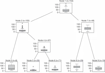
The decision nodes are represented by circles, and each circle is numbered. The input variable to split upon is shown in each circle, together with the P value of the dependence test. For example, the first decision node at the top shows that Temp is the variable that is most strongly associated with Ozone and thus is selected as the first node. The association is measured by a P<0.001. The left and right branches show that a cutoff value equal to 82 is the best to reduce impurity. Thereafter, the decision nodes are further divided by variables Wind and Solar.R sequentially. The leaf nodes show the classifications of Ozone by the decision tree. Because variable Ozone is a continuous variable, the result is displayed by box plot (Figure 1).
Decision tree plot can be modified by setting graphical parameters. For example, if you want to display boxplot, instead of statistics, in inner nodes (decision nodes). The following code can be used:
> plot(airct, inner_panel = node_boxplot, edge_panel = function(...) invisible(),tnex = 1)
As you can see from Figure 2, all inner nodes show boxplot of observations.
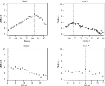
Sometimes investigators are interested in examining the split statistics based on which the split point is derived (4). Remember that the split input variable is continuous variable and there are numerous split points to choose from. For a given split point there is a statistic measuring how good the splitting is. A greater statistic value is associated with a better splitting. Split statistics can be derived from
splitstatistic element of a split. The following syntax draws
scatter plots of split statistics for inner nodes 1, 2, 4 and 7. The leaf nodes have no split statistics because they do not split any more (the tree stops growing at leaf node, Figure 3).
> inner <- nodes(airct, c(1, 2, 4,7))
> layout(matrix(1:length(inner), ncol = length(inner)/2)) > out <- sapply(inner, function(i) {
Figure 1 Conditional inference tree for the airquality data. For each inner node, input variable and P values are given, the boxplot of ozone value is displayed for each terminal node.
Figure 2 Conditional inference tree for the airquality data with the ozone value displayed for both inner and terminal nodes. ≤82
≤81 ≤6.3
≤8
>81 >6.3
>8 >82
1
2
4
7 Wind
P<0.001
Wind P=0.023
Solar.R P=0.023
Temp P<0.001
Node 5 (n=26) Node 8 (n=29) Node 9 (n=19) Node 3 (n=8) Node 6 (n=71)
150
100
50
0
150
100
50
0
150
100
50
0
150
100
50
0
150
100
50
0
Q
-0
8
±
0
�
0 _Q_
k
0 0
-y-1
I
I
E;:J
:
-1-__J_
0 __J_
Node 5 (n=26) Node 8 (n=29) Node 9 (n=19) Node 3 (n=8)
Node 4 (n=97) Node 2 (n=105)
Node 1 (n=153)
Node 7 (n=48)
Node 6 (n=71) 150
100 50 0
150 100 50 0
150 100 50 0
150 100 50 0
150 100 50 0
150 100 50 0
150 100 50 0
150 100 50 0
[image:4.595.114.479.439.694.2]x <- airquality[[i$psplit$variableName]][splitstat >0] p l o t ( x , s p l i t s t a t [ s p l i t s t a t > 0 ] , m a i n = paste("Node",i$nodeID), xlab = i$psplit$variableName, ylab = "Statistic",ylim = c(0, 10), cex.axis = 1.2, cex.lab = 1.2,cex.main = 1.2)
abline(v = i$psplit$splitpoint, lty = 4) })
Prediction with decision tree
The purpose of building a decision tree model is to predict responses in future observations. A subset of the airquality data frame is employed as a new cohort of observations.
> ind <- sample(2, nrow(airquality), replace=TRUE, prob = c(0.7,0.3))
> newData <- airquality[ind==2,]
> newpred <- predict(airct, newdata= newData)
> plot(newpred,newData$Ozone,xlab="Ozone value predicted by decision tree",ylab="Observed ozone value")
The sample() function returns indicator vector of the same length to the row number of the airquality data frame. There are two levels of “1” and “2” in this vector. Observations in the airquality data frame denoted by “2” are selected to constitute the newData. Then the predict() function is used to make a prediction based on input variables. Because the decision tree results in five classifications (5 leaf nodes), the predict() function returns a vector with five values. Each value is the mean value of observations in each leaf nodes (Figure 4). We plot predicted value against observed value in a scatter plot. Not surprisingly, the predicted values take only five values.
Random forests
In the above sections, I grow a single tree for prediction. This method has been criticized for its instability to small changes
10
8
6
4
2
0
10
8
6
4
2
0
10
8
6
4
2
0
10
8
6
4
2
0 60 65 70 75 80 85 90
6 8 10 12 14
60 65 70 75 80 85 90
5 6 7 8 9 10 11 Temp
Statistic
Statistic
Statistic
Statistic
Node 2 Node 1
Wind Wind
Solar.R
[image:5.595.122.476.84.373.2]Node 7 Node 4
in the training data. In recursive partitioning framework, the decision on which input variable to split in and the split point determine how observations are split into leaf nodes. The exact split position and input variable to be selected are highly dependent on the training data. A small change to the training data may alter the first variable to split in, and the appearance of tree can be completely altered. One approach to this problem is to grow a forest instead of one tree (7). Diversity is introduced from two sources: (I) a set of trees is built on random samples of the training sample; and (II) the set of variables to be selected from in each decision node is restricted. Trees of the forest can be built on bootstrap
20 30 40 50 60 70 80
0
20
40
60
80
100
120
Ozone value predicted by decision tree
Observed ozone value
Observed ozone value
Ozone value predicted by decision tree 120
100
80
60
40
20
0
20 30 40 50 60 70 80
Observed ozone value
Predicted ozone value based on random forest 120
100
80
60
40
20
0
20 40 60 8020 40 60 80
0
20
40
60
80
100
120
Predicted ozone value based on random forest
[image:6.595.68.265.82.245.2]Observed ozone value
Figure 4 Scatter plot showing predicted value based on conditional inference tree against observed value. The predicted values are only allowed to take five values that are the mean values of each classification.
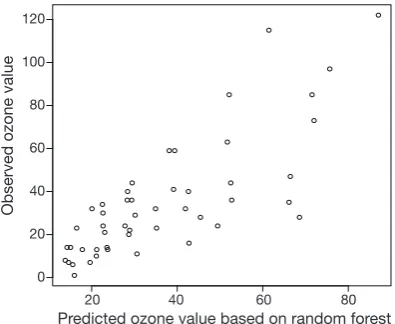
Figure 5 Scatter plot showing the observed ozone values against predicted values by random forests model. This time the predicted value is not restricted to five levels. Instead, they are evenly distributed across the ozone range, which is more likely to occur in the real world.
samples or a subsample of the training dataset. If there are 10 variables to be selected from, we can restrict it to 5 at given split node. The five variables are randomly selected and the pools of candidate variables can be different across forest trees. The final prediction model is the combination of all trees (8).
> aircf<-cforest(Ozone ~ ., data = airquality) > aircf
Random Forest using Conditional Inference Trees Number of trees: 500
Response: Ozone
Inputs: Solar.R, Wind, Temp, Month, Day Number of observations: 153
The syntax for fitting a random forests model is similar to a single conditional inference tree. The output of aircf shows that we have grown 500 trees. The response variable is Ozone and input variables are Solar.R, Wind, Temp, Month and Day. Tree plot cannot be drawn because these trees are different in structure. However, we can make prediction with the random forests model. Again, we use the predict() function, but this time the model is aircf.
> predforest<-predict(aircf, newdata= newData)
> plot(predforest,newData$Ozone,ylab="Observed ozone value",xlab="Predicted ozone value based on random forest")
In the graphical output (Figure 5), observed ozone values are plotted against predicted values by random forests model. This time the predicted value is not restricted to five levels. Instead, they are evenly distributed across the ozone range, which is more likely to occur in the real world.
Model based recursive partitioning
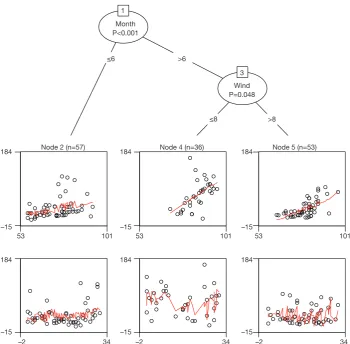
[image:6.595.68.266.310.472.2]Figure 6 Linear-regression-based tree for the airquality data. The leaf nodes give partial scatter plots for Temp (upper panel) and Day (lower panel).
> a i r m o d < - m o b ( O z o n e ~ T e m p + D a y | S o l a r . R+Wind+Month , data = airquality)
> plot(airmod)
In the above code, we used variables Temp and Day to construct a linear regression model with the Ozone as the response variable. Variables after symbol “|” are partitioning variables. The result is displayed with decision tree plot (Figure 6). Because Temp is used as a predictor in regression model, it no longer participates in partitioning. Thus the first partition is made on the variable Month. There seems no strong association between Day and Ozone as shown in the Figure. Therefore, we need to take a close look at statistics of the model.
> airmod
1) Month <= 6; criterion = 1, statistic = 32.402
2)* weights = 57 Terminal node model
Gaussian GLM with coefficients: (Intercept) Temp Day -52.3217 0.9880 0.7325
1) Month > 6
3) Wind <= 8; criterion = 0.952, statistic = 15.979 4)* weights = 36
Terminal node model
Gaussian GLM with coefficients: (Intercept) Temp Day -200.2079 3.1813 -0.1323
3) Wind > 8 5)* weights = 53 184
–15
53 101
–2 34 –2 34 –2 34
53 101 53 101
Node 2 (n=57) ≤6
≤8 >8 >6
1
3
Node 4 (n=36)
Wind P=0.048 Month
P<0.001
Node 5 (n=53)
184
–15
184
–15
184
–15
184
–15
184
Terminal node model
Gaussian GLM with coefficients: (Intercept) Temp Day -149.8501 2.1784 0.5631
The above output displays coefficient of fitted linear regression model. The coefficient of Temp varied remarkably across leaf nodes, indicating a good partitioning. The coefficient of each leaf nodes can be extracted using coef() function.
> coef(airmod)
(Intercept) Temp Day
2 -52.32172 0.9880186 0.7325495 4 -200.20787 3.1812577 -0.1323226 5 -149.85014 2.1783656 0.5630807
The output of coef() function displays model coefficient for each leaf node. Test for parameter stability can be examined with the sctest() function by passing a model based tree and node number to the function.
> sctest(airmod, node =1)
Solar.R Wind Month
statistic 7.3785883 3.016852e+01 3.240226e+01 p.value 0.8682267 1.012705e-04 3.405009e-05
In the above output, we can see that the P value for
Month is the smallest and thus split of the first decision node
is made on Wind (Figure 6).
Summary
The article introduces some basic knowledge on decision tree learning. It employs recursive binary partitioning algorithm that splits the sample in partitioning variable with the strongest association with the response variable. The process continues until some certain criteria are met. In the example I focused on conditional inference tree, which incorporated tree-structured regression models into conditional inference procedures. While growing a single tree is subject to small changes in the training data,
random forests procedure is introduced. The sources of diversity for random forest come from the random sampling and restricted set of input variables to be selected. Finally, I introduce R functions to perform model based recursive partitioning. This method incorporates recursive partitioning into conventional parametric model building.
Acknowledgements
None.
Footnote
Conflicts of Interest: The author has no conflicts of interest to
declare.
References
1. Lantz B, editor. Machine learning with R. 2nd ed. Birmingham: Packt Publishing, 2015.
2. Hothorn T, Hornik K, Zeileis A. Unbiased Recursive Partitioning: A Conditional Inference Framework. Journal of Computational and Graphical Statistics 2006;15:651-74. 3. Zhang Z. Too much covariates in a multivariable model
may cause the problem of overfitting. J Thorac Dis 2014;6:E196-7.
4. Hothorn T, Hornik K, Strobl C, et al. Party: A laboratory for recursive partytioning. 2010.
5. Strasser H, Weber C. On the Asymptotic Theory of Permutation Statistics. SFB Adaptive Information Systems and Modelling in Economics and Management Science, WU Vienna University of Economics and Business, 1999. 6. Zhang Z. Missing data imputation: focusing on single
imputation. Ann Transl Med 2016;4:9.
7. Strobl C, Malley J, Tutz G. An introduction to recursive partitioning: rationale, application, and characteristics of classification and regression trees, bagging, and random forests. Psychol Methods 2009;14:323-48.
8. Breiman L, editor. Random Forests. Machine Learning. Dordrecht: Kluwer Academic Publishers, 2001:5-32. 9. Zeileis A, Hothorn T, Hornik K. Model-Based Recursive
Partitioning. Journal of Computational and Graphical Statistics 2012;17:492-514.