Multivariable control for a three phase rectifier based on deadbeat algorithm

Multivariable Control for a Three-Phase Rectifier

Based on Deadbeat Algorithm

Jaime Rohten§, Pericle Zanchetta ¨, Marco Rivera♠, Javier Muñoz♠, José Espinoza·, José Silva·

§Department of Electrical and Electronic Engineering, Universidad del Bío-Bío, Concepción, Chile, Tel.: +56(41) 311 1566.

¨Department of Electrical and Electronic Engineering, University of Nottingham, U.K. ♠ Department of Industrial Technologies, Universidad de Talca, Chile, Tel.: +56 (75) 220 1746.

·Electrical Engineering Department, University of Concepción, Chile, Tel: +56(41) 220 3512.

JRohten@ubiobio.cl,Pericle.Zanchetta@nottingham.ac.uk, marcoriv@utalca.cl, jamunoz@utalca.cl, jose.espinoza@udec.cl, jsilvac@udec.cl

Abstract—This paper presents a deadbeat control technique

applied in a voltage source rectifier to regulate both the dc voltage (active power) and reactive power injected to the grid. As the deadbeat control is based on the system model, it leads to a faster response, without overshoot and no need to tune the controller parameters. Hence, it is used to fully control the voltage source rectifier, achieving a fast dynamic response for both the dc voltage and the power factor at the point of connection. However, there are some issues related to the high amount of power required to reach the references –especially in the dc voltage­ in a few control steps. The proposed technique also protects the equipment by limiting the maximum power drained to/from the source. The mathematical development is made as a function of the converter power in order to limit it, but at the same time tracking the references with high dynamics, characteristic typical of deadbeat control.

Keywords—Deadbeat Control; Voltage Source Rectifier.

I. INTRODUCTION

Power converters have given significant solutions to the actual industry, providing accurate control of power, voltage and current, in low, medium and high power applications [1], [2]. However, power converters –voltage and current source- exhibit a nonlinear behavior, which complicates the mathematical analysis and their control. Therefore, many control techniques have been developed in order to manage the currents and voltages of power electronic devices [3] – [6]. Despite linear controllers have been already designed for power converters, nonlinear control fits better for these nonlinear systems [7] – [12].

Among recently introduced control techniques, model based predictive control has been successfully applied to power converters, because the model and –consequently- its behavior can be easily found by using the Kirchhoff laws. Finite Control Set-Model Predictive Control (FS-MPC), for example, is based on predicting the system behavior using all possible converter available states and applying at the next sampling time the one that minimizes a specific cost function [8], [9]. However, there are other techniques -also based on predictive control- that do

not use all possible cases to reach the references [7], [10], among them, the deadbeat control [13]-[16].

This paper proposes a novel deadbeat method applied to active rectifiers based on the voltage source converter. Deadbeat control is a technique with significant advantages as fast dynamic response, because it tries to track the references as soon as the model allows, i.e. the reference will be reached depending on the systems order. Traditionally, deadbeat controller is implemented only for current control [9], [11], [12]. This work however suggests a deadbeat approach for the control of whole system in a multivariable configuration, replacing the conventional linear control for the dc voltage.

The employed topology uses a three-phase converter with an RL input filter, which allows to boost the voltage from the ac side to the dc side, which in turn contributes with a second order dynamic in the current behavior. In addition, a dc capacitor is included to storage the power taken from the ac side and to maintain a desired dc voltage level, giving an additional dynamic. Thus, it can be seen that the whole system has a third order response; then, theoretically, the reference can be reached in three sampling steps at most.

Regardless the deadbeat control theory, there are some concerns related to nonlinear power converters, one of them is related with the saturation due to the maximum voltage that can be injected by the power converter, limited by the dc voltage. On the other hand, the maximum power that can be requested by the rectifier is limited by the maximum current that the RL input filter and the switches may bear. Therefore, a power control is also recommended if a deadbeat controller is implemented [9].

Once the current references are established –by the power control and the supply voltage- the converter voltage is selected – based on the model- and synthetized by a space vector modulation technique. The results show the fast dynamic and the minimum overshoot obtained with this technique. Furthermore, the resulting algorithm is easy to implement in a digital environment; thus, the whole analysis is performed in the discrete domain in order to facilitate the digital implementation.

II. POWER CONVERTER MODEL

A. abc Reference Frame Model

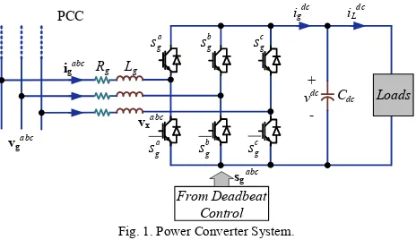
The three-phase Active Front End (AFE) topology used in this work is shown in Fig. 1, where the RL input filter imposes the current dynamics and the dc capacitor the dc voltage dynamics. The voltage Kirchhoff law in the ac side leads to:

v gabc =L dg i gabc/dt+Rgi gabc+vxabc, (1) and formulating the current Kirchhoff law on the dc side:

dc dc dc

C dvdc /dt=ig -iL . (2)

where the current and voltage through the power converter is: abc abc dc dc abcigabc

v x =s g v , i g =sg (3) B. αβ Reference Frame Model

The model can be transformed to the αβ reference frame, in order to reduce the number of equations, for balanced systems. The transformation used is given by:

2 é1 -1/ 2 -1/ 2 ù

3 0 3 / 2 - 3 /

ab₌

x ê 2úxabc, (4)

ë û

where x and x represent the variable in abc and αβ reference frames, respectively. Therefore, the power converter model can be rewritten with the fobllowing equations:

abc αβ

g / g

v gab=L di gab dt R+ i gab+vxab, (5)

. (6)

/

C dc dv dt=s g i g -iL C. Discrete Time Modeling

For digital implementation, it is recommended to discretize the power converter model in order to use these equations on the control design. The most used discretization method is performed through the Euler approximation, and given by:

ab ab

dc dc

( )

(

) (

where x represents the discretized derivate approximation, and Tsthe sampling time. Therefore, the power converter model can

be rewritten, using (7), in the discrete form as:

ab ab

dx t / dt»

(

x k+ -1 x k

)

)

/ Ts, (7)

( )

g

(

k+ -1

)

(k

)

g

( )

(

Ts

k L g R k k

)

,(8)

ab _{= +} ab ₊ ab

g g

i ig

v i vx

(

+ -1

)

(k

)

_{( )}

_{( )}

₍

dc dc

ab ab dc

s i (9)

dc x g

Ts

III. DEADBEAT CONTROL

The aim of the control study is to manage the dc voltage and the power factor at the Point of Common Coupling (PCC). Both of them are related to the power consumed by the converter which, in fact, tie the ac power to the dc power.

A. Desired Voltage Injected by the Converter

The voltage injected by the rectifier named vx can be

calculated from (8) as:

v k v

C = k k -iL k

)

.

( )

( )

(

k+ -1

)

(k

)

(k

)

x g g g

Ts

. (10)

where igαβ (k + 1) can be established as the current reference imposing a given vxαβ (k) to reach this reference in one step ahead. However, due to the impossibility to apply the voltage vxαβ (k) at time k, because of the intrinsic computing delay, the expression (10) must be one step forwarded leading to:

ab ab

v k v k L Rig

ab ab

g

ab ₌ ab _- i ig _- ab

(

)

(

(

)

(

1

)

g ab

ig

(

1

)

g g

Ts

+ =1 +1

)

+

ˆ , (11)

+2 - + _ˆ

k k

k k

-L -R k+

ab ab

x ˆ g

v v

i ig

where the current reference is now given by igαβ (k + 2). On the other hand, a couple of new variables are necessary

αβ

to calculate v x (k + 1). First, an estimation of the current igαβ (k + 1) can be calculated from (8) as:

ab

(

)

(

ab

(

(

s g

)

(

g

( )

( ) (k

)

)

Second, an estimation of thegrid voltage vgαβ (k + 1) can be

ˆ _{+ = -1 1 / }

/ v sg

g s g g

ab ab dc

i k T R L

)

ig k

)

+

T L k - k v . (12)

calculated as v kˆg

(

+ =1

)

ej 2 pf gTsvg

(

k

)

, leading to:



(

)

= ê g

( ) (

s

)

gb

( ) (

Ts

)

ù

( ) (

)

b

( ) (

g s g Ts

)

ú

év k cos wT -v k sin w

k+1

v k sin T v k cos

a ab

a

ê w + w ú

ë û

Voltage vx(k + 1) is a function of the current reference

ig(k + 2), which in turn are imposed by (i) the active power that

charges/discharges the dc capacitor, and (ii) the reactive power, which fixes the power factor at the PCC.

B. Current References

The power supplied by the grid can be separated in active and reactive components, expressed as:

ˆ g

[image:2.595.64.296.51.185.2]

v . (13)

Fig. 1. Power Converter System.

R g Lg

Cdc

PCC

vgabc igabc

igdc iLdc

a

g g g

abc

s sb sc

a b

g g g

s s sc

+

vdc

abc -

vx

Loads

sg From Deadbeat

( )

{



( )

k

)

g g

}

( )

( )

( )

=Re

p k vg k i

g g g



=v a k i× a k +vb k i×gb

(k

)

*

(

, (14)

( )

{



( ) (k

)

}

( )

( )

( )

*

=Im

q k_g v k i_g g

g g g

=vb k i× a k -v a k i×gb

(k

)

, (15)

where vg represents the voltage phasor and ig represents the

current conjugate phasor as:

 *

( )

a

( )

b

( )

_, *

( )

a

( )

g g g g g

. (16)

From (14) and (15), the currents are calculated as a function of the grid voltage and the desired active and reactive power as:

= + =

-v k v k jv k i k i k jigb

(k

)

 

(

( )

( )

( )

(k

)

vg

(k

)

b, ref g



g 2

b ref _- a ref

v k p k vg k q

i k

)

= , (17)

( )

=q

(

k

)

+v

( )

k ig

(

k

)

a b,

ref ref

a, ref g

ig k . (18)

vgb

(

k

)

Equations (17) and (18) give the current as a function of the desired active and reactive power. However, (11) needs the current references at time k + 2; therefore, (17) and (18) must be two step forwarded to use them for the current references. On the other hand, when (17) and (18) are forwarded, it is required the voltage vgαβ (k + 2) which can be found as:

 2 2 

ˆ

(

2

)

j× pf gTs

(

k

)

, (19)

g

and the power references should also be found at step k + 2, leading to:

v k+ =e vg

(

)

=

ig k+2

(

)

(

)

(

)

(

2

)

(

2

)

b, ref g

2

vb k 2 pref k 2 vga k 2 qref k

vg k+

+ + - + +



, (20)

a b,

ref ref

(

)

=

(

)

₍

(

₎

)

(

2

)

a, ref q k 2 vg k 2 ig k

ig k+2 . (21)

vgb k+2

+ + + +

C. Power References

The power references can be separated in (i) the active power reference, defined by the active power consumed by the AFE, and (ii) the injection of the reactive power, defined by the power factor. The active power consumed by the AFE is separated between (a) the dc power, to charge/discharge the dc

dc dc

capacitor and the power consumed by the load v iL , and (b)

the amount of power dissipated by the RL input filter. Thus, (a) the dc active power can be written as:

( )

d v

(

(

t

)

)

2

( )

(

t

)

1

2 dt

or in the discrete form:

dc

dc dc dc

dc

= + × . (22)

p t C v t iL

( )

(

)

2

(k

)

( )

(k

)

2

1 1

2 Ts

and (b) the power used by the first order RL input filter is expressed as:

dc dc

dc dc dc

dc

v k v

p k = C + - +v k i×L , (23)

( )

(

( )

( )

)

 k

)

RL =Re

{

g - x g

}

, (24)

p k v k v k i *

(

where the voltage v k_g

( )

-vx

(

k

)

can be written as:

( )

( )

(k

)

g x g

v k -v k =z ig , (25)



  

with zg= Rg+ jLg. Therefore, the power p RLis now defined as:

( )

{

( )

)

{

(k

)

2

}

( )

{



}

(

 2  2

=Re

}

=Re

=i k Re z =i k

)

Rg

RL g g g g

g g g

Consequently, the active power required by the AFE is:

ref dc

p k z i k i k  z ig

*

(



 

. (26)

(

2

)

(

2

)

RL

(

2

)

this equation is two step forwarded to achieve the desired reference required by (20) and (21). As (27), and therefore (23)

dc

p k+ =p k+ +p k+ , (27)

is two step forwarded, the voltage v (k + 3) is defined as the dc

dc

voltage reference and the voltage vˆ

(

k+2

)

needs to be estimated. A prediction of vdccan be found using (9) as:

(

)

( )

(

(

( )

)

T

( )

(

k

)

)

Cdc

. (28)

From (28) it is easy to note that if this equation is again one

dc

vˆdc k+ =1 vdc k + Ts s gab k i gab k -iLdc

[image:3.595.317.550.48.339.2]

step forwarded –to obtain v (k + 2)- it will be necessary to

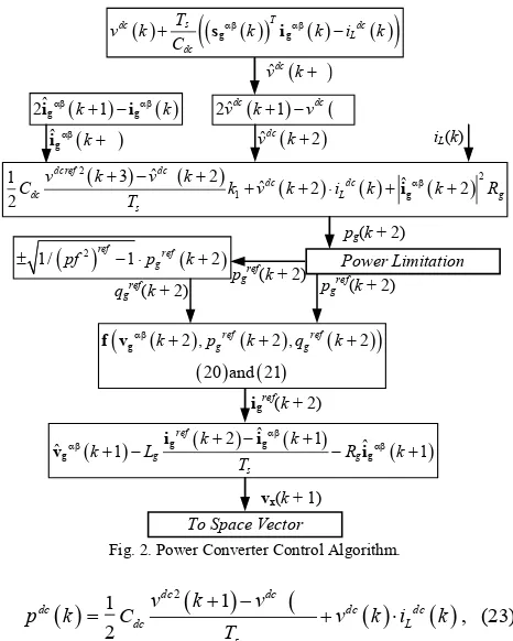
Fig. 2. Power Converter Control Algorithm.

( ) 2( 2) _{( ) ( ) (}

dcref2 dc ₂

1 g

3 ˆ

1 _{ˆ 2 ˆ 2)}

i

2 Ts

dc dc ab

dc L

v k v k

C + - + k +v k+ ×i k + k+ Rg

iL(k)

( )

2 ref( 2)

± 1/ pf ref- ×1 pg k+

( ) ( ) ( 2)

)

(

( ) (21)

+2 , +2 , +

g g

20 and

ab ref ref

f v k p k qg k

qgref(k + 2) pg (k + 2) pg(k + 2)

igref(k + 2)

( _{+ -1}) ref( +2)-ˆab( +1)_- ˆ ( ₊1)

ˆ g g g

Ts

k k

k L g R k

ab i ig ab

v ig

vx(k + 1) To Space Vector

Power Limitation

( )

(

(

( )

)

T ( ) (k)

)

dc Ts ab ab dc

Cdc

v k + s g k i g k -iL

( 1) ˆdc

v k+

ig k+ vˆ (dc k+2)

( ) (k)

2 ˆ_vdc _{k+ -}1 _vdc

( ) ( )

2ˆab k 1 ab k

g +

-i ig

( 2) ˆab

include: (i) i L(k + 1) which normally is defined as a disturbance,

being this prediction a difficult task, then it is considered the

ˆ ˆ

following approximation i_L (k + 2) ≈ iL(k + 1) = iL(k), (ii) the

switching state at step k + 1, which is not feasible because this variable is the controller output, (11). Consequently, to

dc

overcome this problem, vˆ

(

k+2

)

is estimated as:

(

)

(

)

(

ˆdc 2 ˆdc 1 dc 1

)

.

v k+ =v k+ + Dv k+ (29) where_Dvdc

(

k_{+ =}1

)

vˆdc

(

k_{+ -}1

)

vdc

(

k

)

.

On the other hand, the reactive power reference is set as a function of the power factor pf and the desired active power, then, the equation is defined as:

(

)

( )

2

(

2

)

q ref k+2 = ± 1/ pf ref - ×1 pref k+ . (30)

g g

D. Effects of the Fast Imposed Dynamic

Deadbeat Control has important advantages as the fast response, and the minimum overshoot. Furthermore, the desired voltage can be achieved in three steps and the power factor in two steps from (20), (21) and (27). However, three steps for the dc link voltage controller is too fast to be accomplished, because the amount of energy to charge/discharge the dc capacitor may be significant. Therefore, it is important to limit this amount of power to protect the rectifier of high currents, which may damage the components. On the other hand, the power converter has a natural saturation point given by the maximum vxvoltage which is related to the dc link voltage.

Thus, two equations are adapted in order to ensure a slower dynamic response. First, the equation that gives the dc active power is rewritten as:

dc dc

( )

1

(

1

)

2

(k

)

( )

(k

)

2

dc 1

2 Ts

, (31)

where k1 is placed to reduce the amount of power required by the first term in (31). This constant also allows to smooth the dynamic response, because it reduces the noise influence on the power reference. This harmful effect is amplified because the voltage is squared and divided by Ts. Then, it is important to

include k1 for noisy variables.

dc v k v dc dc

p k = C + - k +v k i×L

The second equation given by (27) needs to be limited in order to reduce the maximum reference current in (20) and (21)

ref pref

. Therefore, the final algorithm states that if p > pmax, then

ref ref

= pmax; and if p < -p max, then p = -p max. The whole control

algorithm is presented in Fig. 2.

IV. VOLTAGE SYNTHETIZATION

Once the voltage vxis defined by the deadbeat control, it

must be synthetized by a modulation technique, [12]. Space Vector is chosen to achieve the requested voltage vxprovided

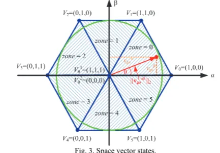
by the deadbeat control. The range of voltages that the modulating strategy is capable to generate can be seen in Fig. 3, limited by the dc link voltage and the eight valid states. Thus, any voltage vxinside the hatched region can be achieved with

the three nearest voltages (one of them the zero state). Thus the voltage vxis synthetized as,

ab ab dc ab dc ab

(

Tsv x =Vi v T1+Vi+1 v T2+Vq Ts- -T1 T2

)

,

where Vθ represents the zero state and i represents the zone where the vector vxis, Fig. 3. Therefore, each state is applied

during the following times:

(32)

(

(

Vi+1

) (

vx

)

1 s

+1

dc ab

)

´ ab

dc dcV

i i

v

T = T , (33)

v _V ab _´ v ab

2

i+1 +1

a dc

x i

s dc dcVi

v v Va

T = T T

v V a -v a 1, (34)

where Viαβis defined as:

(

)

(

3

)

23

= ésin × p/ 3 cos × p/ ùT

iab _ë i i _û

Now, in order to decide the zone where the voltage vxis

V , (35)

placed, Fig. 3, the angle θ = arg{vxαβ (k + 1)} is calculated as:

æ ö

(

vxa

(k

+1

)

(

1

)

è 2ø

q =_sign

(

_{vx k}+₁

)

)

×_arccosç ÷ ç _vx k+ ÷

b

ab , (36)

TABLE I PARAMETERS

Parameters Value

vg 230 V, rms

v dc 600 V Rg 0.4 Ω

Lg 4.75 mH C dc 2.2 mF Rdc 250 Ω

fg 50 Hz

fs 10kHz

k1 0.06

V. RESULTS

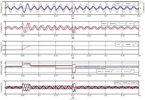
[image:4.595.65.282.53.204.2] [image:4.595.315.551.284.388.2]

The designed controller is tested under dc voltage reference step change, Fig. 4. The dc voltage changes from 600V to 650 V in t = 0.05 s and then it goes back to 600V in t = 0.2 s. The results illustrated in Fig. 4 show that the reference is achieved in only 20 ms approximately for the step up, i.e. one grid cycle, for a 50 V step change. In addition, it is worth to highlight that no overshoot is presented, which is an advantage of the deadbeat control. On the other hand, the time to reach the reference when it goes down is less than when it goes up, which is mainly due to the losses presented in the inverter, making easier to reduce instead to increase the power stored in the dc capacitor.

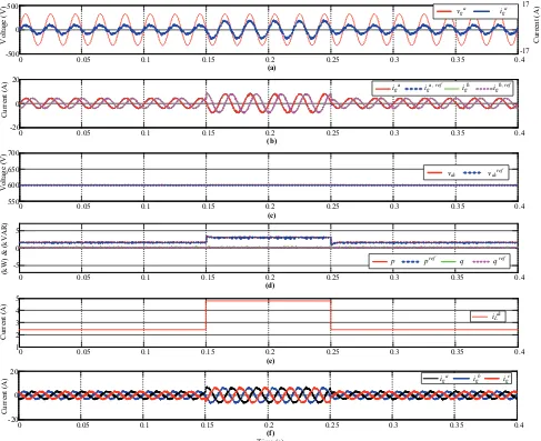
Aiming to see the load impact behavior, Fig. 5 shows the system response when the dc current is incremented in a 100% from 2.4 A. This was obtained inserting a 250 Ω resistor in parallel to R dc= 250 Ω. The result shown in Fig. 5 describes that

the dc voltage as well as the power factor is maintained in their reference value even with this significant step change, and the deadbeat control imposes higher currents in order to track its references given by the requested load power.

VI. CONCLUSIONS

Deadbeat control is a suitable alternative to control power converters. When this method is applied on this multivariable systems, the time response is significantly reduced, and without

overshoot. On the other hand, and despite the fast response, the maximum amount of power is limited by the same algorithm protecting the equipment of potential damage due to extreme operating conditions. In addition, as the control algorithm is based on the model, it is intuitive once the variables and references are defined.

REFERENCES

[1] S. Yang, A. Bryant, P. Mawby, D. Xiang, L. Ran and P. Tavner, "An Industry-Based Survey of Reliability in Power Electronic Converters,"

in IEEE Transactions on Industry Applications, vol. 47, no. 3, pp. 1441-

1451, May-June 2011.

[2] Q. Chen, "Opportunities and challenges to power electronics industry in alternative and renewable energy," Power Electronics Systems and

Applications, 2009. PESA 2009. 3rd International Conference on, Hong

Kong, 2009, pp. 1-1.

[3] P. Gaur and P. Singh, "Various control strategies for medium voltage high power multilevel converters: A review," Engineering and Computational Sciences (RAECS), 2014 Recent Advances in, Chandigarh, 2014, pp. 1- 6.

[4] P. Kowstubha, K. Krishnaveni and K. Ramesh Reddy, "Review on different control strategies of LLC series resonant converters," Advances

in Electrical Engineering (ICAEE), 2014 International Conference on,

Vellore, 2014, pp. 1-4.

[image:5.595.62.551.51.387.2]

[5] S. Debnath, J. Qin, B. Bahrani, M. Saeedifard and P. Barbosa, "Operation, Control, and Applications of the Modular Multilevel Converter: A Review," in IEEE Trans. on Power Electron., vol. 30, no. 1, pp. 37-53, Jan. 2015.

Fig. 4. Power control loops v step and reactive power control (a) grid voltage and current, (b) reference and measured αβ grid current, (c) reference and measured abc.

dc

dc voltage, (d) reference and measured active and reactive power, and (e) grid currents ig

0 0.05 0.1 0.15 0.2 0.25 0.3 0.35 0.4

(a)

-500 0 500

Vo

lt

ag

e

(V)

0 0.05 0.1 0.15 0.2 0.25 0.3 0.35 0.4

(b)

-20 0 20

C

urre

nt

(A

)

0 0.05 0.1 0.15 0.2 0.25 0.3 0.35 0.4

(c)

650

600

550 700

Vo

lt

ag

e

(V)

a a

vg ig

iga iga , ref i gß igß , ref

vdcref

vdc

-17 17

0

Cur

re

nt

(A

)

0 0.05 0.1 0.15 0.2 0.25 0.3 0.35 0.4

(e)

Time (s)

0 0.05 0.1 0.15 0.2 0.25 0.3 0.35 0.4

(d)

-5 5

0

-20 0 20

Cur

rent (

A

)

(k

W

)

&

(k

VA

R

)

iga igb igc

pref q ref

[6] J. Muñoz, J. Rohten, J. Espinoza, P. Melín, C. Baier and M. Rivera, "Review of current control techniques for a cascaded H-Bridge STATCOM," Industrial Technology (ICIT), 2015 IEEE International

Conference on, Seville, 2015, pp. 3085-3090.

[7] P. Cortés, M. Kazmierkowski, R. Kennel, D. Quevedo, and J. Rodríguez “Predictive Control in Power Electronics and Drives,” IEEE Trans. on

Ind. Electron., vol. 55, no 12, pp. 4312–4324, Dic. 2008.

[8] M. Pérez, M. Vásquez, J. Rodríguez, J. Pontt, “FPGA-based predictive current control of a three-phase active front end rectifier”, in Conf. Rec.

IEEE ICIT’12, pp. 1–6, Feb. 2009.

[9] J. Rohten, J. Espinoza, J. Munoz, D. Sbarbaro, M. Pérez, P. Melin, J. Silva, E. Espinosa, “Enhanced Predictive Control for a Wide Time Variant Frequency Environment” IEEE Trans. on Ind. Electron., vol. PP, no 99, pp. 1, Mar. 2016.

[10] Y. Zhang, W. Xie, Y. Zhang, “Deadbeat direct power control of three- phase pulse-width modulation rectifiers” IET Power Electronics, vol. 7, no 6, pp. 1340–1346, Nov. 2013.

[11] M. Pérez, M. Vásquez, J. Rodríguez, J. Pontt, “Research on deadbeat Current Control Strategy of Three-Phase PWM Voltage Source Rectifier”, in Conf. Rec. IEEE ICIT’12, pp. 1–6, Feb. 2009.

[12] C. Xia, M. Wang, Z. Song, and T. Liu, “Robust Model Predictive Current Control of Three-Phase Voltage Source PWM Rectifier with Online Disturbance Observation” IEEE Trans. on Ind. Informatics, vol. 8, no 3, pp. 459–471, Mar. 2012.

[13] Y. Zhang, W. Xie and Y. Zhang, "Deadbeat direct power control of three- phase pulse-width modulation rectifiers," in IET Power Electronics, vol. 7, no. 6, pp. 1340-1346, June 2014.

[14] A. Luo, H. Xiao and Z. Shuai, "Double deadbeat-loop control method for distribution static compensator," in IET Power Electronics, vol. 8, no. 7, pp. 1104-1110, 7 2015.

[15] K. Nishida, T. Ahmed and M. Nakaoka, "Cost-Effective Deadbeat Current Control for Wind-Energy Inverter Application With Filter," in

IEEE Trans. on Industry Applications, vol. 50, no. 2, pp. 1185-1197,

March-April 2014.

[image:6.595.63.550.53.450.2]

[16] Z. Xueguang, Z. Wenjie, C. Jiaming and X. Dianguo, "Deadbeat Control Strategy of Circulating Currents in Parallel Connection System of Three- Phase PWM Converter," in IEEE Transactions on Energy Conversion, vol. 29, no. 2, pp. 406-417, June 2014.

Fig. 5. Step load impact (a) grid voltage and current, (b) reference and measured αβ grid current, (c) reference and ameasured dc voltage, (d) reference and

abc abc.

measured active and reactive power, (e)dc load current i L , and (f) grid currents ig

V

ol

tag

e

(V

)

V

olt

age (

V

)

Cur

re

nt (

A

)

(e)

C

urre

nt

(A

)

(f) (d)

(kW) &

(kV

A

R)

-17 17

C

ur

re

nt (

A

)

Time (s)

Cur

rent (

A

)

0 0.05 0.1 0.15 0.2 0.25 0.3 0.35 0.4

(a)

-500 0 500

0 0.05 0.1 0.15 0.2 0.25 0.3 0.35 0.4

(b)

-20 0 20

0 0.05 0.1 0.15 0.2 0.25 0.3 0.35 0.4

(c)

600

550 700

650

a a

vg ig

iga i ga , ref i gß igß , ref

vdcref

vdc

0 0.05 0.1 0.15 0.2 0.25 0.3 0.35 0.4

-5 5

0

pref q ref

p q

0 0.05 0.1 0.15 0.2 0.25 0.3 0.35 0.4

-20 0 20

i ga i gb igc

0 0.05 0.1 0.15 0.2 0.25 0.3 0.35 0.4

3 2 1 5

4 dc

iL