EFFICIENT SCHEDULING OF WORKFLOW IN CLOUD ENVIORNMENT USING BILLING MODEL AWARE TASK CLUSTERING

SPEAKER RECOGNITION IN CLEAN AND NOISY

ENVIRONMENT USING RBFNN AND AANN

1_{R. VISALAKSHI,} 2_{P. DHANALAKSHMI}

1_{Assistant Professor, Department of Computer Science and Engineering} 2_{Associate Professor, Department of Computer Science and Engineering}

E-mail: [email protected], [email protected]

ABSTRACT

In this paper, we propose a speaker recognition system based on features extracted from the speech recorded using close speaking microphone in clean and noisy environment. This system recognizes the speakers from a number of acoustic features that include linear predictive coefficients (LPC), linear predictive cepstral coefficients (LPCC) and Mel-frequency cepstral coefficients (MFCC). RBFNN and AANN are two modelling techniques used to capture the features. RBFNN model enables nonlinear transformation followed by linear transformation to achieve a higher dimension in the hidden space. The proposed work compares the performance of RBFNN with Autoassociative neural network (AANN). The autoassociative neural network (AANN) is used to capture the distribution of the acoustic feature vectors in the feature space. This model captures the distribution of the acoustic features of a class, and the backpropagation learning algorithm is used to adjust the weights of the network to minimize the mean square error for each feature vector. The experimental results show that, the performance of AANN performs better than RBFNN. AANN gives an accuracy of 94.93% for various acoustic features both in clean and noisy environment.

Keywords: Radial Basis Function Neural Network (RBFNN); Autoassociative Neural Network (AANN); Linear Predictive Coefficients (LPC); Linear Predictive Cepstral Coefficients (LPCC); Mel-Frequency Cepstral Coefficients (MFCC); Speaker Recognition (SR)

1. INTRODUCTION

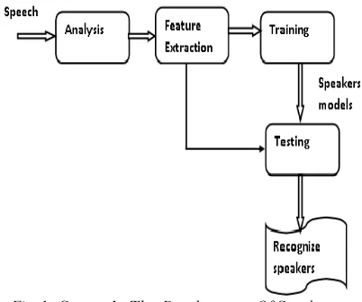
As speech interaction with computers becomes more pervasive in activities such as financial services and information retrieval from speech databases, the utility of automatically recognizing a speaker based solely on vocal characteristics increases. Given a speech sample, speaker recognition is concerned with extracting clues to the identity of the person who was the source of that utterance [3]. Speaker recognition is divided into two specific tasks: verification and identification [4]. In speaker verification the goal is to determine from a voice sample if a person is whom he or she claims. In speaker identification the goal is to determine which one of a group of knowing voices best matches the input voice sample. In either case the speech can be constrained to a known phrase dependent) or totally unconstrained (text-independent) [9] In most of the applications voice is used to confirm the identity claim of a speaker. Speaker recognition system may be viewed as working on four stages namely Analysis, Features Extraction, Modeling and Testing as shown in Fig.1.

Fig. 1 Stages In The _Development _{Of Speaker}

Recognition System

∑

= ∧

−

−

=

k

k

s

n

k

a

n

s

1

)

(

)

(

system. The physical structure and dimension of the vocal tract as well as the excitation source are unique for each speaker. This uniqueness are embedded in the speech signal during speech production and can be used for speaker recognition. To obtain a good representation of these speaker characteristics, speech data needs to be analyzed. The speech analysis stage deals with the selection of suitable frame size and frame shift for segmenting the speech signal for further analysis and feature extraction [2].

1.1. Outline of the Work

In order to distinguish the two categories of speech data from clean and noisy environment, the features are extracted using linear prediction analysis (LPC), Linear Prediction Cepstral Coefficients (LPCC) and Mel frequency Cepstral

Coefficients (MFCC). The three layer radial basis function neural network (RBFNN) model as described in Section.3.1 is used to capture the distribution of the feature vectors. The RBFNN model is used for capturing the distribution of the acoustic features of a class, and the k-mean clustering algorithm is used to adjust the weights of the network to minimize the mean square error for each feature vector. The performance of RBFNN is compared to AANN feed forward neural network. The auto associative neural network (AANN) is used to capture the distribution of the acoustic feature vectors in the feature space. This model captures the distribution of the acoustic feature of a class and the back propagation learning algorithm is used to adjust the weights of the network to minimize the mean square error for each feature vector. Experimental results show that the accuracy of AANN with Mel-frequency cepstral features can provide a better result. Fig. 2 Illustrates the block diagram of speaker recognition.

Fig:2 Block Diagram Of Speaker Recognition

The paper is organized as follows. The feature extraction techniques are presented in Section 2. Modeling techniques for speaker recognition is

RBFNN and AANN are reported in Section 4. Finally, conclusions and future work are given in Section 5.

2.ACOUSTIC FEATURE EXTRACTION TECHNIQUES

Preprocessing

To extract the features from the speech signal, the signal must be pre-processed and divided into successive windows or analysis frames. Throughout this work, sampling rate of 8 kHz, 16 bits

monophonic, pulse code modulation (PCM) format in wave speech is adopted [7]. Speech signal which is recorded using a close-speaking microphone from the collected speaker database speech data is pre-processed before extracting features. This involves the detection of begin and end points of the utterance in the speech waveform, pre-emphasis and windowing of the frame. The process of pre-emphasis provides high frequency emphasis and windowing reduces the effect of discontinuity at the ends of each frame of speech. The speech samples in each frame are pre-processed using a different operator to emphasize the high frequency components.

2.1 Linear Prediction Analysis

For acoustic feature extraction, the difference speech signal is divided into frames of 20ms, with a shift of 10 ms. A pt h order LP analysis is used to capture the properties of the signal spectrum.

In the LP analysis of speech each sample is predicted as the linear weighted sum of the past p

samples, where p represents the order of prediction[10]. If s(n) is the present sample, then it is predicted by the past p samples as

(1)

2.2 Mel-frequency cepstral coefficients

The extraction and selection of the best parametric representation of acoustic signals is an important task in the design of any speech recognition system; it significantly affects the

recognition performance [1]. A compact

are proving more efficient. The calculation of the MFCC includes the following steps.

Mel-frequency Wrapping

Human perception of frequency contents of sounds of speech signal does not follow a linear scale. Thus for each tone with an actual frequency f, measured in Hz, a subjective pitch is measured on a scale called the Mel scale. The Mel-frequency scale is linear frequency spacing below 1KHz and a logarithmic spacing above 1kHz. As a reference point, the pitch of a 1 KHz tone, 40dB above the perceptual hearing threshold, is defined as 1000 mels. Therefore, we can use the following approximate formula to compute the mels for a given frequency f in Hz.

= (2)

Where F_mel is the logarithmic scale of f normal frequency scale.

3. MODELING TECHNIQUES FOR SPEAKER RECOGNITION

3.1 Radial basis function neural network model

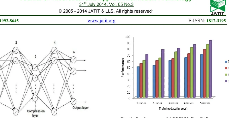
The radial basis function neural network (RBFNN)[8] has a feed forward architecture with an input layer, a hidden layer and an output layer as shown in Fig. 3. Radial basis functions are embedded into a two-layer feed forward neural network. Such a network is characterized by a set of inputs and a set of outputs. In between the inputs and outputs, there is a layer of processing units called hidden units. Each of them implements a radial basis function. RBFNN solves the classification problem by transforming the input space into a high dimensional space in a non-linear manner. The RBFNN uses a Gaussian basis function as the radial basis function in the hidden layer. The significance of the radial basis function is that the output is a function of radial distance [6]. The Gaussian basis function of the hidden unit for an input vector ( ) is given by

= exp (3)

The and are calculated by using a suitable clustering algorithm

Fig.3 Radial Basis Function Neural Network

3.2 Autoassociative neural network models

.

Fig.4 Autoassociative Neural Network Models.

During training the target vectors are same as the input vectors. The AANN trained with a data set will capture the subspace and the hypersurface along the surface of maximum variance of the data [14].

4. EXPERIMENTAL RESULTS 4.1 Datasets

The evaluation of the proposed speaker recognition system is performed by using a speech database which consists of the following contents: Recording was done in the laboratory under clean and noisy environment. Speech from volunteers

was acquired using the close-speaking

microphones for 2 secs to 5 secs. The data obtained from each of the 400 speakers is used to train a speaker model. Each test utterance was about 2 secs to 5 secs duration. The recordings for training and testing the speaker models were carried out in separate sessions.

4.2 Modeling using RBFNN

In RBFNN training, 14 LPC, 19 LPCC and 39 MFCC features are extracted from the speech data that can later be used to represent each speaker. These features are given as input to RBFNN model. The RBF centers are located using k-means algorithm. The weights are determined using a least squares algorithm. The value of k = 1,

2 and 5 has been used in our studies for two categories. The system gives optimal performance for k= 5. The value of k = 1 to 5 has been used in

our studies for each speaker. The system gives optimal performance for k=5. The performance of RBFNN for different means shown in Fig 6.

Fig. 6 Performance Of RBFNN For Different Mea_ns.

Table 1: Speaker Recognition Performance Using RBFNN

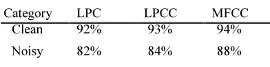
For training, the weight matrix is calculated using the K-mean clustering algorithm as discussed above. For speaker recognition the feature vectors are extracted and each of the feature vector is given as input to the RBFNN model. The average output is calculated for each of the output neuron. The class to which the speech sample belongs is decided based on the highest output. A comparison with the performance of speaker recognition between two categories for the feature vectors using LPC, LPCC and MFCC for RBFNN is given in Table 1.

4.3Modeling using AANN

The five layer autoassociative neural network model as described in Section 3.3, is used to capture the distribution of the acoustic feature vectors. The structure of the AANN model used in our study is 14L 38N 4N 38N 14L for LPC, 19L 38N 4N 38N 19L for LPCC, 39L 78N 4N 78N 39L for MFCC, for capturing the distribution of the acoustic features of a class, where L denotes a linear unit, and N denotes a nonlinear unit. The nonlinear units use tanh(s) as the activation function, where s is the activation value of the unit. The backpropagation learning algorithm is used to adjust the weights of the network to minimize the mean square error for each feature vector. The speech signals are recorded for 2 sec to 5 sec at 8000

Category LPC LPCC MFCC

Clean 90% 91% 92%

msec, with a shift of 10 msec. A 14t h order LP analysis is used to capture the properties of the signal spectrum as described in Section 2. The recursive relation [12] between the predictor

coefficients and cepstral coefficients is used to convert the 14 LP coefficients into 19 cepstral coefficients. The LP coefficients for each frame is linearly weighted to form the LPCC. The distribution of the 14 dimensional LPC feature vectors, 19 dimensional LPCC feature vectors and 39 dimensional MFCC feature vectors in the feature space is captured using an AANN model.

TABLE 2:Speaker Recognition Performance Using AANN

Separate AANN models are used to capture the distribution of feature vectors of each class. The distribution is usually different for different speaker[12]. The acoustic feature vectors are given as input to the AANN model and the network is trained for 300 epochs. One epoch of training is a single presentation of all the training vectors to the network. The AANN training process creates a separate model for each category For testing, the speech signal is recorded for 2 sec to 5 sec. For evaluating the performance of the system, the feature vector is given as input to each of the models. The output of the model is compared with the input to compute the normalized squared error. The normalized squared error (E) for the feature

vector y is E , where o is the output vector

given by the model. The error (E) is transformed into a confidence score (C) using C = exp (−E ).

The average confidence score is calculated for each model. The class is decided based on the highest confidence score. The performance of the system is evaluated , and the method achieves about 94.93%.

Table 3:Speaker Recognition Performance Using RBFNN And AANN

RBFNN AANN

89.1% 94.93%

LPC, LPCC and MFCC for AANN is given in Table 2. The performance of the system using RBFNN and AANN for speaker recognition is given in Table 3.

5. CONCLUSION

In this paper, we have proposed a speaker recognition system using RBFNN and AANN model. LPC, LPCC and MFCC features are extracted from the voice signal or speech data that can later be used to represent each speaker.

Experimental results show that, then

Characteristics of the speech data are collected from clean and noisy environment using close speaking microphone. The speaker information present in the source features is captured using RBFNN and AANN model. RBFNN method may provide robustness against channel and handset effects, which are known to degrade the performance of a speaker recognition system. The degradation in performance is due to the change in speaker characteristics. We used AANN models to train the noisy speech, which ensures that the voice characteristics of the speaker is similar in both the training and testing stage. By comparing the results of the two models, AANN performs better and shows an accuracy of 94.93%. In future, throat microphone can be used for speaker recognition.

REFRENCES:

[1] T. Vibha, Mfcc and its applications in speaker

recognition, International Journal on

Emerging Technologies, 2010.

[2] P. Rupali, Kulkarni .M, Analysis of FFSR, VFSR, MFSR techniques for feature extraction in speaker recognition: a review. IJCSI , 7 (4): 1694–0814.

[3] K. Tomi, Li H (2010) An overview of text

independent speaker recognition: From

features to supervectors. ScienceDirect, Speech Communication, 2010.

[4] D.A. Reynolds An overview of automatic speaker recognition technology. ICASSP , 2002.

[5] S. Haykin Neural networks a comprehensive foundation, (Pearson Education, 2001b, Asia). [6] S. Haykin Neural networks a comprehensive

foundation, (Pearson Education, 2001a, Singapore).

Category LPC LPCC MFCC

Clean 92% 93% 94%

[7] L. Rabiner, Juang B Fundamentals of Speech Recognition, (Pearson Education, Singapore, 2003).

[8] B. Yegnanarayana, Artificial neural networks, Prentice Hall of India, 1999, New Delhi. [9] B. Yegnanarayana, S.V. Gangashetty, S.

Palanivel Autoassociative neural network models for pattern recognition tasks in speech and image. In: Soft Computing Approach to Pattern Recognition and Image Processing, World Scientific publishing Co. Pte. Ltd, Singapore, pp 283–305, 2002.

[10]N. Balakrishnan, Improved Text-Independent Speaker Recognition using Gaussian Mixture Probabilities, M.S thesis, Carnegie Mellon university, 2005

[11] P. Dhanalakshmi (2010) Classification of audio for retrieval applications, Ph.D thesis, AU, Chidambaram, August 2010.

[12]B. Yegnanarayana, Reddy K.S, Kishore S.P,

Source and system features for speaker recognition using a model. In: IEEE Int. Conf. Acoust., Speech and Signal Processing, Salt Lake City, Utah, USA, pp 409–412, 2001. [13]B. Yegnanarayana, Kishore S, AANN: an

alternative to GMM for pattern recognition. Neural Networks, 15:459–469, 2002.

[14]M. S. Ikbal, Misra H, Yegnanarayana B,