SOLVING ECONOMIC DISPATCH PROBLEM USING PARTICLE SWARM OPTIMIZATION BY AN EVOLUTIONARY TECHNIQUE FOR INITIALIZING PARTICLES

(1)

MODELING OF THE PART DYNAMICS OF THE MIDWATER

TRAWL BASED ON R LANGUAGE

1, 2, 3_{YUWEI LI,} 1, 2, 3_{XINFENG ZHANG,} 1, 2, 3_{XIAORONG ZOU,} 1, 2, 3_{MIN ZHANG,} 1, 2, 3_XINJUN

CHEN, 1, 2, 3LIUXIONG XU, 1, 2, 3LIMING SONG, 1, 2, 3YINGQI ZHOU

1_{College of Marine Sciences, Shanghai Ocean University, Shanghai 201306, China}

2_{The Key Laboratory of Sustainable Exploitation of Oceanic Fisheries Resources, Ministry of Education,}

Shanghai Ocean University, Shanghai 201306, China

3

National Engineering Research Centre for Oceanic Fisheries, Shanghai Ocean University,

Shanghai 201306, China

ABSTRACT

In this study, the part dynamics of the midwater trawl were modeled and simulated using mechanical equations and R language. A lumped mass method was used to model the dynamical behavior of a net in steady flow. And the implicit algorithm was developed to solve the stiff differential equations. The programming, simulation and visualization of the modeling were based on the R platform. The part dynamics of the trawl in the sea water were presented successfully, and the motion process conformed well to the observed data in the ocean.

Keywords: Implicit Method, Trawl Net, Numerical Modeling, R Language, Lumped Mass Method

1. INTRODUCTION

Midwater trawl is a kind of big fishing gear to catch fish which lives in the midwater layers in the Ocean. In recent years, the fishing gear design of midwater trawl has improved based on the water tank experiments and the development of mechanical research. But nonlinear differential equations, derived from the fishing gears, are difficult to solve. Few studies have addressed fishing gears by numerical simulation models. Hu et al. described the dynamical analysis of midwater trawl system with two-dimensional lumped mass method [1]. Priour et al. described trawl net shapes by the finite element method with triangular elements [2-4]. Takagi et al. used the lumped mass method to study the fishing gear system by subdividing the elements of fishing gears [5]. Lee et al. used an implicit calculation method to simulate trawl gear with the lumped mass method [6].

However, the computation of the models are too complex and difficult to understand due to the complicated structure. The coordinated systems used in the calculation are most the local coordinate systems and need to be converted. Most of the nonlinear differential equations are solved by the explicit method such as Runge-Kutta method. But they suffer from instability and accuracy problems,

and the time step of stable solution is extremely limited by the stiffness of the flexible engineering systems [7].

R is an implementation of the S programming language combined with lexical scoping semantics inspired by Scheme, and is created by Ross Ihaka and Robert Gentleman at the University of Auckland, New Zealand [8]. Although R is a programming language and software environment for statistical computing and graphics, it can also be used as a general matrix calculation toolbox with performance benchmarks comparable to MATLAB [9]. Berend Hasselman has developed a package (nleqslv) to solve the systems of no linear equations [10]. It is capable to be used to some simple initial value problems of ordinary differential equations. For some complicated engineering systems (such as the modeling of big fishing gears with hundreds of higher-order differential equations), it shows much weakness. The mathematical modeling of the dynamics of trawl is just the performance of a complicated engineering system.

(2)

Real-Time Visualization Device System for R (RGL) was also used to display the 3D dynamical process.

2. METHODS

2.1 Numerical Modeling of Part Dynamics of Trawl

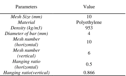
In this study, considering the part shape of trawl, a virtual mathematical mesh model with 10 by 6 meshes was established (Fig.1 and Table.1). The trawl system is composed of nettings, ropes, floats, sinkers, otter board and other affiliations. Many mathematical models considered fishing gear systems as flexible systems, which are the physical systems with many lumped mass point interconnected by springs. In our model, mass points are considered to be concentrated at each knot and the midpoint of each mesh bar. To simplify the model, an assumption was that no external force exist on the spring. There only exists the forces of tension force acted on the spring, and gravity, buoyancy and hydrodynamic force (drag force and lift force) acted on the mass points. And the four corners of the net are fixed.

[image:2.612.92.298.476.601.2]

Figure 1: The Schematic Diagram Of Mesh Model

Table 1 : The Net Materials Used In The Model

Parameters Value

Mesh Size (mm) 10

Material Polyethylene

Density (kg/m3) 953

Diameter of bar (mm) 4

Mesh number

(horizontal) 10

Mesh number

(vertical) 6

Hanging ratio

(horizontal) 0.5

Hanging ratio(vertical) 0.866

2.2 Equations of Mechanical Models

It was assumed that the fishing net was in a state with spatial-temporally uniform current flow. The motion of point i can be expressed by the following equation based on the Newton second law:

i

M a= + + +T F W B

r r r r

(1)

Where a is the acceleration vector of point i; T is the tension force acting on point i; F is the hydrodynamic force including drag force and lift force; W is the gravity force; B is the buoyancy

force, and M is the mass of point i including the added mass of i.

Each mesh knot was considered with a spherical shape (Fig.2). Hence the fluid dynamical coefficients in all directions are the same. The dynamical equations of knot i are:

i i x x i i y y

i i z z i i

M x T F

M y T F

M z T F W B

 _{= +}



= +

 

= + − +



&& &&

&&

(2)

Where x&&_i , &&y_i and z_&&_i are the second-order derivatives of the location coordinates of x, y and z.

The mesh bar is looked as a spring, based on the Hooke's law, the tension T could be expressed as:

0

0 0

0

| |

0

ij ij

ij ij ij ij

ij

ij ij

l l

EA l l

l T

l l

−



>



=

 _≤



(3)

Where A ,_ij E are cross sectional area and the modulus of elasticity of the mesh bar between mass points i and j, respectively.l and_0ij l are the original _ij

length and deformed length between mass points i and j, respectively. Then the model of tension force can be obtained as:

( )

| |

( )

| |

( )

| |

j i

x ij

j H ij j i

y ij

j H ij j i

z ij

j H ij

x x

T T

l

y y

T T

l

z z

T T

l ∈

∈

 ₋

=

 

 ₋



=

 

 ₋

 ₌



∑

(4)

Where H indicates the number of neighboring points arrounding the i-th point.

Figure 2: The Schematic Diagram Of The Knot

(3)

1 | | ( ) 2 1 | | ( ) 2 1 | | ( ) 2

x d i i

y d i i

z d i i

F C S x u x u

F C S y v y v

F C S z w z w

ρ ρ ρ = − − = − − = − − & & & & & & (5)

Where, ρis the density of water; C_dis the drag coefficient, Sis the projection area of point i and (u, v, w) --the water flow velocity in three dimensions. The dot-notation (•) represents differentiation of the first order with respect to time t. So the dynamical equations of point i were:

1 1 1 ( , , , , , , ; ) ( , , , , , , ; ) ( , , , , , , ; )

i i i i i j j j i i i i i j j j i i i i i j j j

x f x y z x x y z t

y g x y z y x y z t

z h x y z z x y z t

= = = && & && & && & (6)

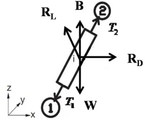
Each mesh bar was assumed to be a cylindrical element (Fig.3). It was assumed that the angles of the bar to the axes of X, Y and Z are

α

,β ,

γ

,

respectively. Then the drag force (R_D ) and lift force (R_L) can be expressed as:

3 90 3 90 3 90 1

(sin ) ( )

2 1

(sin ) ( )

2 1

(sin ) ( )

2

Dx N f i i

Dy N f i i

Dz N f i i

R dl C C x u x u

R dl C C y v y v

R dl C C z w z w

ρ α π

ρ β π

ρ γ π

 = + − −    = + − −    = + − −   & & & & & & (7)

Where is the diameter of the mesh bar; is the original length of mesh bar; is the drag coefficient in the state that the flow is vertical to the bar; and is the resistance coefficient caused by viscous force (Table.2); is the projection component.

[image:3.612.126.271.529.648.2]

Figure 3: The Schematic Diagram Of The Mesh Bar

Table 2 : The Coefficient Parameters Used In The Model

Parameters Value

CN90 1.20

cf 0.0064

Cm 1.0

g(m/s2) 9.81

density of water(kg/m3₎ ₁₀₃₀

v(m/s) 10.0

Cd 0.47

E 28500000

2 90 2 90 2 90 2 90 2 90 2 1

(sin cos )| |( ) 2

1

(sin cos )| |( ) 2

1

(sin cos )| |( ) 2

1

(sin cos )| |( ) 2

1

(sin cos )| |( ) 2

1 (sin 2

Lx N i i

N i i

Ly N i i

N i i

Lz N i i

R dl C z w z w

dl C y v y v

R dl C z w z w

dl C x u x u

R dl C y v y v

dl

ρ γ γ ξ

ρ β β ξ

ρ γ γ ξ

ρ α α ξ

ρ β β ξ

ρ = − − + − − = − − + − − = − − + & & & & & & & & & & 90

cos CN )|xi u| (xi u)

α α ξ

               − − 

 & &

(8)

For the equations of tension force, the formula is similar to equations (3) and (4). The motion of the i-th bar can be expressed as:

( )

i i x Dx Lx i i y Dy Ly

i i z Dz Lz i i

M x T R R

M y T R R

M z T R R B W

 ₌ ₊ ₊  = + +   = + + + −  && && && (9)

Equation (9) can be changed into ordinary differential equations:

2 1 1 1 2 2 2

( , , , , , , , , , , , ; ) ( , , , , , , , , , , , ; ) ( , , , , , , , , , , , ; )

i i i i i i i

x f x y z x y z x y z x y z t

y g x y z x y z x y z x y z t

z h x y z x y z x y z x y z t

= = =

&& & & & && & & &

& & && &

(10)

2.3 Programming, Algorithm and Simulation

The equations (6) and (10) are implicit and high-order ordinary differential equations. In high-order to resolve directly in R, we define

i i

x& =q ,y&_i =u_i,z&_i =h_i. Then (6) and (10) could be converted to first-order differential equations:

1 1 1 ( , , , , , , ; ) ( , , , , , , ; ) ( , , , , , , ; )

i i i i i j j j i i i i i j j j i i i i i j j j

q f x y z q x y z t

u g x y z u x y z t

h h x y z h x y z t

= = = & & & (11)

2 1 1 1 2 2 2

( , , , , , , , , , , , ; ) ( , , , , , , , , , , , ; ) ( , , , , , , , , , , , ; )

i i i i i i i

q f x y z q u h x y z x y z t

u g x y z q u h x y z x y z t

h h x y z q u h x y z x y z t

= = = & & & (12)

(4)

time t of the motion of net is divided into T steps, k ≤T. And dt is time step and dt=t[k+1]-t[k]. And we used the improved euler method to calculate the equation (13). Then the improved euler method is used as:

[ 1] [ ]

[ 1]

[ 1] [ ] ( [ ] [ 1] ) 2

[ 1] [ ] ( ( ) ( 1) ) 2

[ 1] [ ] ( ( ) ( 1

2

m m

i i i i

m m

i i i i

m m

i i i i

m m

i i i i

m

i i i i

dt

x k x k q k q k

dt

y k y k u k u k

dt

z k z k h k h k

dt

q k q k f k f k

dt

u k u k g k g k

+

+ = + × + +

+ = + × + + [ ]

[ 1] [ ]

) ) [ 1] [ ] ( ( ) ( 1) )

2

m

m m

i i i i

dt

h k+ + =h k + ×h k +h k+

(13)

Where m is the m-th step of iterations for implicit Euler iterative computation.

The above algorithm is used to compile the program and to calculate the models in the R platform. These equations are solved numerically at all given points using a workstation. After that, the dynamics of part of the trawl net under sea water can be simulated.

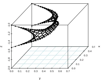
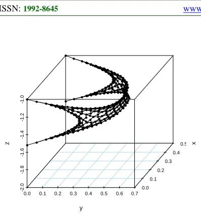
3. VISUALIZATION OF THE RESULTS

After modeling and programming the part of trawl net using mechanical equations and implicit algorithm under R platform, another graphical package of R was used to visualize the results. The package 3D Real-Time Visualization Device System for R (RGL) is very powerful and it can exhibit the dynamics successfully and vividly in three dimensions. The results of the simulation and visualization presented lively the extending process from the initial position to the equilibrium state (Fig. 4, 5, 6 and 7) and the motion process conformed well to the observed data in the ocean. Due to the large size of figures, we only gave some important figures to exhibit the dynamical process of the part behavior of trawl net under the sea water. Zhang et al. researched the part behavior of purse seine using half-implicit algorithm [11].

0.0 0.1 0.2 0.3 0.4 0.5 0.6 0.7

-2

.0

-1

.8

-1

.6

-1

.4

-1

.2

-1

.0

0.0 0.1

0.2 0.3

0.4 0.5

y

x

[image:4.612.330.522.324.471.2]

z

Figure 4: The Initial Shape Of The Part Of Midwater Trawl

0.0 0.1 0.2 0.3 0.4 0.5 0.6 0.7

-2

.0

-1

.8

-1

.6

-1

.4

-1

.2

-1

.0

0.0 0.1

0.2 0.3

0.4 0.5

y

x

[image:4.612.331.522.539.691.2]

z

Figure 5: Beginning To Extend By The Flow Of Sea Water

0.0 0.1 0.2 0.3 0.4 0.5 0.6 0.7

-2

.0

-1

.8

-1

.6

-1

.4

-1

.2

-1

.0

0.0 0.1

0.2 0.3

0.4 0.5

y

x

z

(5)

0.0 0.1 0.2 0.3 0.4 0.5 0.6 0.7

-2

.0

-1

.8

-1

.6

-1

.4

-1

.2

-1

.0

0.0 0.1

0.2 0.3

0.4 0.5

y

x

[image:5.612.92.291.73.294.2]

z

Figure 7: The Equilibrium State Of Part Of Midwater Trawl

The present study gave another new successful case that lumped mass method, implicit algorithm and R language can be integrated to solve complicated engineering system.

4. CONCLUSION

Lumped mass method was a high efficient method in simulating the part of midwater trawl. The implicit and high-order ordinary differential equations could be solved by improved euler method and R language could quickly perform the operation. The present study could be applied in other complicated fishing gears.

ACKNOWLEDGEMENTS

This work was supported by1) Shanghai Leading Academic Discipline Project (No.S30702); 2) Key technology in high efficient utilization of Chilean jack mackerel (Trachurus murphyi)resources (No. 2012AA092301); 3) Key technology in pelagic tuna's purse seine fishing and ultralow temperature preservation (No. 2012AA092302); 4) Technical development in fishing and processing of squid resources (No. 2012AA092303); 5) Shanghai Municipal Education Commission Innovation Project (No. 12ZZ168).

REFERENCES:

[1] F. X. Hu, K. Matuda, T. Tokai,and K. Haruyuki, “Dynamic analysis of midwater trawl system by a two dimensional lumped mass method”,

Fisheries Sciences, Vol. 61, No. 2, 1995, pp.

229-233.

[2] D. Priour, “Calculation of net shapes by the finite element method with triangular elements”,

Communications in Numerica1 Methods, Vol.

15, No. 10, 1999, pp. 755-763.

[3] D. Priour, “ Introduction of mesh resistance to opening in a triangular element for calculation of nets by the finite element method”,

Communications in Numerical Methods in Enginering, Vol. 17, No. 4, 2001, pp. 229-237.

[4] D. Priour, “Analysis of nets with hexagonal mesh using triangular element”, Numerical methods

in engineering, Vol. 56, No. 12, 2003, pp.

1721-1733.

[5] T. Takagi, T. Shimizu, K. Suzuki, T. Hiraishi,K. Yamamoto, “Validity and layout of “NaLA”: a net configuration and loading analysis system” ,

Fisheries Reseach, vol. 66, No. 2-3, 2004, pp.

235-243.

[6] C. W. Lee, J. H. Lee, B. J. Cha, H. Y. Kim, and J. H. Lee, “Physical modeling for underwater flexible systems dynamic simulation”, Ocean

Engineering, Vol. 32, No. 3-4, 2005, pp. 331–

347.

[7] C. W. Lee, J. H. Lee, ”Modeling of a midwater trawl system with respect to the vertical movements”, Fisheries Science, Vol. 66, No. 5, 2000, pp.851-857.

[8] http://myprofile.cos.com/rgentleman. [9] http://www.sciviews.org/benchmark.

[10] http://cran.csie.ntu.edu.tw/web/packages/nleqslv /index.html.