Kernel Partial Least Squares for Stationary Data
Marco Singer [email protected]
Institute for Mathematical Stochastics Georg-August-Universit¨at
G¨ottingen, 37077, Germany
Tatyana Krivobokova [email protected]
Institute for Mathematical Stochastics Georg-August-Universit¨at
G¨ottingen, 37077, Germany
Axel Munk [email protected]
Institute for Mathematical Stochastics Georg-August-Universit¨at
G¨ottingen, 37077, Germany
Editor:Sara van de Geer
Abstract
We consider the kernel partial least squares algorithm for non-parametric regression with stationary dependent data. Probabilistic convergence rates of the kernel partial least squares estimator to the true regression function are established under a source and an effective dimensionality condition. It is shown both theoretically and in simulations that long range dependence results in slower convergence rates. A protein dynamics example shows high predictive power of kernel partial least squares.
Keywords: effective dimensionality, long range dependence, nonparametric regression, source condition, protein dynamics
1. Introduction
Partial least squares (PLS) is a regularized regression technique developed by Wold et al. (1984) to deal with collinearities in the regressor matrix. It is an iterative algorithm where the covariance between response and regressor is maximized at each step, see Helland (1988) for a detailed description. Regularization in the PLS algorithm is obtained by stopping the iteration process early.
Several studies showed that partial least squares algorithm is competitive with other regression methods such as ridge regression and principal component regression, needing generally fewer iterations than the latter to achieve comparable estimation and prediction, see, e.g., Frank and Friedman (1993), Kr¨amer and Braun (2007) and Singer et al. (2016). For an overview of further properties of PLS we refer to Rosipall and Kr¨amer (2006).
Reproducing kernel Hilbert spaces (RKHS) have a long history in probability and statis-tics (see, e.g., Berlinet and Thomas-Agnan, 2004). Here we focus on the supervised kernel based learning approach for the solution of non-parametric regression problems. RKHS methods are both computationally and theoretically attractive, due to the kernel trick
c
(Sch¨olkopf et al., 1998) and the representer theorem (Wahba, 1999), as well as its gener-alization (Sch¨olkopf et al., 2001). Within the reproducing kernel Hilbert space framework one can adapt linear regularized regression techniques like ridge regression and principal component regression to a non-parametric setting, see Saunders et al. (1998) and Rosipal et al. (2000), respectively. We refer to Sch¨olkopf and Smola (2001) for more details on the kernel based learning approach.
Kernel PLS (KPLS) was introduced in Rosipal and Trejo (2001) by using the reformu-lation of the PLS algorithm of Lindgren et al. (1993). The rereformu-lationship to kernel conjugate gradient (KCG) methods was highlighted in Blanchard and Kr¨amer (2010a). It can be seen in Hanke (1995) that conjugate gradient methods are well suited for handling ill-posed problems, as they arise in kernel learning, see, e.g., De Vito et al. (2006).
Rosipal (2003) investigated the performance of kernel partial least squares for non-linear discriminant analysis. Blanchard and Kr¨amer (2010a) proved the consistency of KPLS when the algorithm is stopped early without giving convergence rates.
Caponnetto and de Vito (2007) showed that kernel ridge regression (KRR) attains op-timal probabilistic rates of convergence for independent and identically distributed data, using a source and a polynomial effective dimensionality condition. A generalization of these results to a wider class of effective dimensionality conditions and extension to kernel principal component regression can be found in Dicker et al. (2017).
For independent identically distributed data Blanchard and Kr¨amer (2010b) obtained probabilistic convergence rates for a certain kernel conjugate gradient estimator under early stopping, while Lin and Zhou (2017) considered kernel partial least squares estimators with the cross-validation stopping rule.
In contrast to existing works, we derive probabilistic convergence rates of the kernel partial least squares estimator to the true regression function when the input data are not independent and identically distributed, but rather stationary time series. To the best of our knowledge, none of the kernel regression methods have been considered for the dependent data so far. Our results can be applied to stationary dependence structures, given that certain concentration inequalities for these data hold. The derived convergence rates depend not only on the complexity of the target function and of the data mapped into the kernel space, but also on the persistence of the dependence in the data. For measuring the complexity of the data we consider general effective dimensionality conditions. In a Gaussian setting we prove that the short range dependence still leads to optimal rates, but if the dependence is more persistent, the rates become slower. We illustrate the good predictive performance of KPLS by an application to the molecular dynamics of a bacteriophage protein.
2. Kernel Partial Least Squares
Consider the non-parametric regression problem
yt=f∗(Xt) +εt, t∈Z. (1)
Let X be a random vector that is independent of Xt t∈Z and εt t∈Z with the same distribution asX0. The target function we seek to estimate is f∗∈ L2 PX
. For the purpose of supervised learning assume that we have a training sample
{(Xt, yt)}nt=1 for some n ∈ N. In the following we introduce some basic notation for the kernel based learning approach.
Define with (H,h·,·iH) the RKHS of functions on Rd with reproducing kernel k:Rd×
Rd→R, i.e., it holds
g(x) =hg, k(·, x)iH, x∈Rd, g∈ H. (2)
The corresponding inner product and norm inHis denoted byh·,·iHand k · kH, respec-tively. We refer to Berlinet and Thomas-Agnan (2004) for examples of Hilbert spaces and their reproducing kernels. In the following we deal with reproducing kernel Hilbert spaces which fulfill the following, rather standard, conditions:
(K1) His separable,
(K2) There exists aκ >0 such that|k(x, y)| ≤κ for all x, y∈Rd andk is measurable.
Under (K1) the Hilbert-Schmidt norm k · kHS for operators mapping from H to H is well defined. If condition (K2) holds, all functions inHare bounded, see Berlinet and Thomas-Agnan (2004), chapter 2. The conditions are satisfied for a variety of popular kernels, e.g., Gaussian or triangular.
The main principle of RKHS methods is the mapping of the data Xt into H via the
feature maps φt = k(·, Xt), t = 1, . . . , n. This mapping can be done implicitly by using
the kernel trick hφt, φsiH =k(Xt, Xs) and thus only the n×n dimensional kernel matrix
Kn=n−1[k(Xt, Xs)]nt,s=1 is needed in the computations. Then the task for RKHS methods is to find coefficientsα1, . . . , αnsuch thatfα =Pnt=1αtφt is an adequate approximation of
f∗ inH, measured in the L2 PX
norm k · k2.
There are a variety of different approaches to estimate the coefficients α1, . . . , αn,
in-cluding kernel ridge regression, kernel principal component regression and, of course, kernel partial least squares. The latter method was introduced by Rosipal and Trejo (2001) and is the focus of the current work.
It was shown by Kr¨amer and Braun (2007) that the KPLS algorithm solves
b
αi = arg min v∈Ki(Kn,y)
n−1ky−Knvk2, i= 1, . . . , n, (3)
with y = (y1, . . . , yn)T. Here Ki(Kn, y) = span
y, Kny, Kn2y, . . . , Kni−1y , i = 1, . . . , n, is
theith order Krylov space with respect toKnand y andk · k denotes the Euclidean norm.
The dimensioniof the Krylov space is the regularization parameter for KPLS.
We will introduce several operators that will be crucial for our further analysis. Define two integral operators: the kernel integral operatorT∗ :L2 PX
→ H, g7→E{k(·, X)g(X)} and the change of space operator T :H → L2 PX
, g 7→ g, which is well defined if (K2) holds. It is easy to see that T, T∗ are adjoint, i.e., for u ∈ H and v ∈ L2 PX
it holds hT∗v, uiH=hv, T ui2 with h·,·i2 being the inner product in L2 PX
.
The sample analogues of T, T∗ are Tn : H → Rn, g 7→ {g(X1), . . . , g(Xn)}T and Tn∗ :
Rn→ H,(v1, . . . , vn)T 7→n−1Pnt=1vtk(·, Xt), respectively. Both operators are adjoint with
respect to the rescaled Euclidean productn−1uTv,u, v∈
Finally, we define the sample kernel covariance operator Sn =Tn∗Tn :H → H and the
population kernel covariance operator S =T∗T :H → H. Note that it holds Kn =TnTn∗.
Under (K1) and (K2)S is a self-adjoint compact operator with operator norm kSkL ≤κ, see Caponnetto and de Vito (2007).
With this notation we can restate (3) for the function fα
f
b
αi = arg min g∈Ki(Sn,Tn∗y)
n−1ky− {g(X1), . . . , g(Xn)}Tk2 = arg min g∈Ki(Sn,Tn∗y)
n−1ky−Tngk2. (4)
Hence, we are looking for functions that minimize the squared distance toy constrained to a sequence of Krylov spaces.
In the literature of ill-posed problems it is well known that without further conditions on the target functionf∗ the convergence rate of the conjugate gradient algorithm can be arbitrarily slow, see Hanke (1995), chapter 3.2. One common a-priori assumption on the regression function f∗ is a source condition:
(S) There existr≥0,R >0 and u∈ L2 PX
such thatf∗ = (T T∗)ru and kuk
2≤R. If r ≥ 1/2, then the target function f∗ ∈ L2 PX
coincides almost surely with a function f ∈ H and we can write f∗ =T f, see Cucker and Smale (2002). With this the kernel partial least squares estimatorfαib estimates the correct target function, not only its
best approximation inH. This case is known as the inner case.
The situation with r < 1/2 is referred to as the outer case. Under additional assump-tions, e.g., the availability of additional unlabeled data, it is still possible that an estimator of f∗ converges to the true target function in L2 PX
norm with optimal rates (with re-spect to the number n of labeled data points). See De Vito et al. (2006) for a detailed description of this semi-supervised approach for kernel ridge regression in the independent and identically distributed case. We do not treat the case r <1/2 in this work.
A source condition is often interpreted as an abstract smootheness condition, see, e.g., Bissantz et al. (2007) for several examples. This can be seen as follows. Letη1 ≥η2 ≥. . . be the eigenvalues andψ1, ψ2, . . . the corresponding eigenfunctions of the compact operatorS. Then it is easy to see that the source condition (S) is equivalent tof =P∞
j=1bjψj ∈ L2 PX
with bj such that P∞j=1η
−2(r+1/2)
j b2j < ∞. Hence, the higher r is chosen the faster the
sequence {bj}∞j=1 must converge to zero. Therefore, the sets of functions for which source conditions hold are nested, i.e., the larger r is the smaller the corresponding set will be. The set with r = 1/2 is the largest one and corresponds to a zero smoothness condition, i.e., P∞
j=1η −2
j b2j <∞, which is equivalent to f ∈ H. For more details we refer to Dicker
et al. (2017).
3. Consistency of Kernel Partial Least Squares
The KCG algorithm as described by Blanchard and Kr¨amer (2010b) is consistent when stopped early and convergence rates can be obtained when a source condition (S) holds. Here we will proof the same property for KPLS. Early stopping in this context means that we stop the algorithm at somea=a(n)≤nand consider the estimator f
b
αa forf∗.
The difference between KCG and KPLS is the norm which is optimized. The kernel conjugate gradient algorithm studied in Blanchard and Kr¨amer (2010b) estimates the co-efficients α ∈Rn of f
α via αb
CG
see that this optimization problem can be rewritten for the function fα as
min
g∈Ki(Sn,Tn∗y)
n−1kTn∗y−Sngk2H = min
g∈Ki(Sn,Tn∗y)
n−1kTn∗(y−Tng)k2H,
compared to (4) for KPLS. Thus, KCG obtains the least squares approximation g in the H-norm for the normal equation Tn∗y =Tn∗Tng and KPLS finds a function that minimizes
the residual sum of squares. In both methods the solutions are restricted to functions
g∈ Ki(Sn, Tn∗y).
An advantage of the kernel conjugate gradient estimator is that concentration inequali-ties can be established for bothTn∗yandSnand applied directly as the optimization function
contains both quantities. The stopping index for the regularization can be chosen by a dis-crepancy principle as a∗ = min{1 ≤ i ≤ n : kSnf
b
αCG
i −T
∗
nyk ≤ Λn} with Λn being a
threshold sequence that goes to zero as nincreases.
On the other hand, the function to be optimized for KPLS contains only y and Tng=
{g(X1), . . . , g(Xn)}T for which statistical properties are not readily available. Thus, we
need to find a way to apply the concentration inequalities for Tn∗y and Sn to this slightly
different problem. This leads to complications in the proof of consistency and a rather different and more technical stopping rule for choosing the optimal regularization parame-tera∗is used, as can be seen in Theorem 1. This stopping rule has its origin in Hanke (1995).
In the following k · kL denotes the operator norm and k · kHS is the Hilbert-Schmidt norm.
Theorem 1 Assume that conditions (K1), (K2), (S) hold with r ≥ 3/2 and there are
constants Cδ(ν), C(ν) > 0 and a sequence {γn}n∈N ⊂[0,∞), γn → 0, such that we have
for ν ∈(0,1]
P (kSn−SkL≤Cδ(ν)γn)≥1−ν/2,
P (kTn∗y−SfkH≤C(ν)γn)≥1−ν/2.
Define the stopping index a∗ by
a∗= min (
1≤a≤n:
a
X
i=0
kSnfαib −T
∗
nyk
−2
H ≥(Cγn)−2
)
, (5)
with C=C(ν) +κr−1/2(r+ 1/2)R{1 +Cδ(ν)}.
Then it holds with probability at least 1−ν that
kf
b
αa∗ −f
∗k 2 =O
n
γn2r/(2r+1)o,
kf
b
αa∗−fkH=O
n
γn(2r−1)/(2r+1)
o
,
with f∗ =T f.
The theorem yields two convergence results, one in theH-norm and one in theL2 PX -norm. It holds that kvk2 = kS1/2vkH. These are the endpoints of a continuum of norms kvkβ =kSβvkH,β ∈[0,1/2] that were considered in Nemirovskii (1986) for the derivation of convergence rates for KCG algorithms in a deterministic setting.
The convergence rate of the kernel partial least squares estimator depends crucially on the sequenceγn and the source parameterr. Ifγn=O(n−1/2), this yields the same
conver-gence rate as Theorem 2.1 of Blanchard and Kr¨amer (2010b) for kernel conjugate gradient or de Vito et al. (2005) for kernel ridge regression with independent and identically dis-tributed data. For stationary Gaussian time series we will derive concentration inequalities in the next section and obtain convergence rates depending on the source parameterr and the range of dependence. Note that Theorem 1 is rather general and it can be applied to any kind of dependence structure, as long as the necessary concentration inequalities can be established.
The next theorem derives faster convergence rates under assumptions on the effective dimensionality of operator S, which is defined as dλ = tr{(S +λ)−1S}. The concept of
effective dimensionality was introduced in Zhang (2003) to get sharp error bounds for general learning problems considered there. IfHis a finite dimensional space, it was shown in Zhang (2003) thatdλ≤dim(H). For infinite dimensional spaces it describes the complexity of the
interactions between data and reproducing kernel.
If dλ = O(λ−s) for some s ∈ (0,1], Caponnetto and de Vito (2007) showed that the
order optimal convergence rates n−r/(2r+s) are attained for KRR with independent and identically distributed data.
The effective dimensionality clearly depends on the behaviour of eigenvalues of S. If these converge sufficiently fast to zero, nearly parametric rates of convergence can be achieved for reproducing kernel Hilbert space methods, see, e.g., Dicker et al. (2017). In par-ticular, the behaviour ofdλaround zero is of interest, since it determines how ill-conditioned
the operator (S+λ)−1 becomes. In the following theorem we set λ =λn for a sequence
{λn}n∈N⊂(0,∞) that converges to zero.
Theorem 2 Assume that conditions (K1), (K2), (S) hold with r≥1/2and that the
effec-tive dimensionality dλ is known. Additionally, there are constantsCδ(ν), C(ν), Cψ >0and
a sequence {γn}n∈N⊂[0,∞), γn→0, such that forν ∈(0,1] and nsufficiently large
P{kSn−SkL≤Cδ(ν)γn} ≥1−ν/3,
Pnk(S+λn)−1/2(Tn∗y−Sf)kH≤C(ν)
p
dλnγn
o
≥1−ν/3,
Pnk(S+λn)1/2(Sn+λn)−1/2kL≤Cψ
o
≥1−ν/3,
Here {λn}n∈N⊂(0,∞) is a sequence converging to zero such that for n large enough
γn≤λrn−1/2. (6)
Take ζn= max{
p
λndλnγn, λ r+1/2
n } Define the stopping index a∗ by
a∗ = min (
1≤a≤n:
a
X
i=0
kSnfαib −Tn∗yk
−2
H ≥(Cζn)−2
)
with C= 4R , Cψ,(r 1/2)κ Cδ(ν),2 R CψC(ν .
Then it holds with probability at least 1−ν that
kfαab ∗ −f
∗k 2 =O
n
λ−1n /2ζn
o
,
kf
b
αa∗ −fkH=O
λ−1n ζn ,
with f∗ =T f.
The condition (6) holds trivially for r = 1/2 as γn converges to zero. For r > 1/2 the
sequence λn must not converge to zero arbitrarily fast.
In its general form Theorem 2 does not give immediate insight in the probabilistic convergence rates of the kernel partial least squares estimator. Therefore, we state two corollaries, where the function dλ is specified. In both corollaries we explicitly state the
choice of the sequenceλn that yield the corresponding rates.
Corollary 3 Assume that there exists s∈(0,1] such that dλ =O(λ−s) for λ→ 0. Then
under conditions of Theorem 2 with λn = γn2/(2r+s) it holds with probability at least 1−ν
that
kf
b
αa∗ −f
∗k 2 =O
n
γn2r/(2r+s)o.
Polynomial decay of the effective dimensionality dλ = tr{(S+λ)−1S} occurs if the
eigen-values of S also decay polynomially fast, that is, µi = csi−1/s for s ∈ (0,1], since in this
case dλ =
∞ P
i=1
{1 +λ/csi1/s}−1 = O(λ−s). This holds, for example, for the Sobolev
ker-nel k(x, y) = min(x, y), x, y ∈ [0,1] and data that are uniformly distributed on [0,1], see Raskutti et al. (2014).
If γn=n−1/2, then the KPLS estimator converges in the L2 PX
-norm with a rate of
n−r/(2r+s). This rate is shown to be optimal in Caponnetto and de Vito (2007) for KRR with independent identically distributed data.
Note that the rate obtained in Theorem 1 corresponds to γn−2r/(2r+s) with s = 1, i.e.,
the worst case rate with respect to the parameter s∈(0,1].
In the next corollary to Theorem 2 we assume that the effective dimensionality behaves in a logarithmic fashion.
Corollary 4 Let dλ =O{log(1 +a/λ)} for λ→0 and a >0. Then under the conditions
of Theorem 2 with λn=γn2log{γn−2}and r= 1/2it holds with probability at least1−ν that
kf
b
αa∗ −f
∗k 2 =O
γnlog(1/2γn−2) .
The effective dimensionality takes the special form considered in this corollary, for example, when the eigenvalues of S decay exponentially fast. This holds, for example, if the data are Gaussian and the Gaussian kernel is used, see Section A. If γn = O(n−1/2), then the
convergence rate is of order O{n−1log(n)}, which is nearly parametric. It is noteworthy that the source condition only impacts the choice of the sequence λn, not the convergence
rates of the estimator in theL2 PX
which is a minimal smoothness condition on f∗, i.e., that f∗ = T f almost surely for an
f ∈ H.
The rates obtained in Corollaries 3 and 4 for γn = n−1/2 were derived in Dicker et al.
(2017) for kernel ridge regression and kernel principal component regression under the as-sumption of independent and identically distributed data.
4. Concentration Inequalities for Gaussian Time Series
Crucial assumptions of Theorem 1 and 2 are the concentration inequalities for Sn and
Tn∗y and convergence of the sequence {γn}n∈N. Here we establish such inequalities in a Gaussian setting for stationary time series. At the end of this section we will state explicit convergence rates for f
b
αa∗ that depend not only on the source parameterr ≥1/2 and the
effective dimensionalitydλ, but also on the persistence of the dependence in the data.
The Gaussian setting is summarized in the following assumptions
(D1) (Xh, X0)T∼ N2d(0,Σh), h= 1, . . . , n−1, with
Σh =
τ0 τh
τh τ0
⊗Σ.
Here Σ ∈ Rd×d and V = [τ|i−j|]ni,j=1 ∈ Rn×n are positive definite, symmetric ma-trices and ⊗ denotes the Kronecker product between matrices. Furthermore X0 ∼ Nd(0, τ0Σ).
(D2) For the autocorrelation function ρh = τ0−1τh there exists a q > 0 such that |ρh| ≤
(h+ 1)−q forh= 0, . . . , n−1.
Condition (D1) is a separability condition for the covariance matrices Σh,h= 0, . . . , n−1.
Due to (D1) the effects (on the covariance) over time and between the different variables can be treated separately. Under condition (D2) it is easy to see that fromq >1 follows the absolute summability of the autocorrelation functionρand thus{Xt}t∈Zis a short memory process. Stationary short memory processes keep many of the properties of independent and identically distributed data, see, e.g., Brockwell and Davis (1991).
On the other hand q ∈ (0,1] yields a long memory process, see, e.g., Definition 3.1.2 in Giraitis et al. (2012). Examples of long memory processes are the fractional Gaussian noise with an autocorrelation function that behaves like (h+ 1)−2(1−H), with H ∈ [0,1) being the Hurst coefficient. Stationary long memory processes exhibit dependencies between observations that are more persistent, and many statistical results that hold for independent and identically distributed data, turn out to be false. See Samorodnitsky (2007) for more details.
The next theorem gives concentration inequalities for both estimators Sn and Tn∗y in
a Gaussian setting with convergence rates depending on the parameter q > 0. These inequalities are the ones needed in Theorem 1 and Theorem 2. Recall that dλ = tr{(S+
Theorem 5 (i) Define dµh(x, y) = dP (x, y) dP (x)dP (y). Under Assumptions
(K1) and (K2) it holds forν ∈(0,1] with probability at least 1−ν that
kSn−Sk2L≤ 2ν−1
n2
n−1 X
h=1
(n−h) Z
R2d
k2(x, y)dµh(x, y) +
ν−1 n
E{k2(X0, X0)} − kSk2HS
,
kTn∗y−Sfk2 H≤
2ν−1 n2
n−1 X
h=1
(n−h) Z
R2d
k(x, y)f(x)f(y)dµh(x, y)
+ν −1
n
Ek(X0, X0)f2(X0) − kSfk2H+σ2E{k2(X0, X0)}
.
(ii) Assume that additionally to (K1), (K2) also (D1), (D2) for q > 0 are fulfilled.
Denote M = supx∈Rd|f(x)|.
Then there exists a constant C(q)>0 such that
kSn−SkL≤ν−1/2{γn2(q)κCγ+n−1(κ2− kSk2HS)}1/2, kTn∗y−SfkH≤ν−1/2γn2(q)M Cγ+n−1
κ(M +σ2)− kSfk2 H
1/2 ,
for Cγ = C(q){(2π)ddet(Σ)}−1/2κd1/2(1−4−q)−1/4(d+2). The function γn(q), q > 0, is defined as
γn(q) =
n−1/2 , q >1
n−1/2log(1/2n) , q= 1
n−q/2 , q ∈(0,1).
(iii) Let (K1), (K2) and (S) hold. Let γn(q) be the function as defined in (ii). Then
there exists a constant C˜ >0such that it holds with probability at least1−ν for λ >0that
k(S+λ)−1/2(Tn∗y−SnfkH≤ν−1/2C˜σ
p
dλγn(q).
(iv) Let (K1), (K2), (S), (D1) and (D2) hold. Let λ−1n /2dλn1/2γn(q) → 0 for a sequence
λn→0 andγn(q) the function defined in (ii). Then there exists ann0 =n0(ν, q)∈N such
that with probability at least 1−ν we have for alln≥n0
k(S+λn)1/2(Sn+λn)−1/2kL≤ √
2.
The first part of the theorem is general and can be used to derive concentration inequal-ities not only in the Gaussian setting and is of interest in itself. The convergence rate is controlled by the sums appearing on the right hand side. If these sums are of O(n), then the mean squared error of bothSnandTn∗ywill converge to zero with a rate ofn−1. On the
other hand, if the sums are of order O(n2−q) for some q ∈(0,1), the mean squared errors
will converge with the reduced rate n−q.
The second part derives explicit concentration inequalities in the Gaussian setting de-scribed by (D1) and (D2) with rates depending on the range of the dependence measured by q >0. These inequalities appear in Theorem 1.
Parts (iii) and (iv) give the additional probabilistic bounds needed to apply Theorem 2. The conditionλ−1n /2dλn1/2γn(q)→0 in Theorem 5 (iv) is fulfilled in the settings of Corollary
3 and Corollary 4.
Corollary 6 Let the conditions of Theorem 2 and (D1), (D2) hold.
(i) Assume that there exists s ∈ (0,1] such that dλ = O(λ−s) for λ → 0. Then with
probability at least 1−ν
kf
b
αa∗ −f
∗k 2 =
O{n−r/(2r+s)}, q >1, O{n−qr/(2r+s)}, q∈(0,1).
If instead of conditions of Theorem 2, conditions of Theorem 1 are assumed, then the
convergence rates above have s= 1.
(ii) Assume that there exists a > 0 such that dλ = O{log(1 +a/λ)} for λ → 0 and
r= 1/2. Then with probability at least 1−ν
kf
b
αa∗ −f
∗k 2 =
O{n−1/2log(1/2n)}, q >1, O{n−q/2log(1/2nq)}, q∈(0,1).
Hence, for q > 1 the kernel partial least squares algorithm achieves the same rates as if the data were independent and identically distributed. Forq ∈(0,1) the convergence rates become substantially slower, highlighting that dependence structures that persist over a long time can influence the convergence rates of the algorithm.
5. Simulations
To validate the theoretical results of the previous sections, we conducted a simulation study. The reproducing kernel Hilbert space is chosen to correspond to the Gaussian kernel
k(x, y) = exp(−lkx−yk2), x, y ∈
Rd, l = 2, for d = 1. Our data will also be normally distributed. We refer to Proposition 7 in Appendix A for the derivation of functions that fulfill the source condition in this setting. Proposition 8 shows that the the eigenvalues of
S decay exponentially fast. Hence the effective dimensionalitydλ behaves as in Corollary 4
and thus we expect convergence rates as given by Corollary 6 (ii).
The source parameter is taken to be r= 4.5 and we consider the function
f(x) = 4.37−1{3L4(x,−4)−2L4(x,3) + 1.5L4(x,9)}, x∈R.
The normalization constant is chosen such thatf takes values in [−0.35,0.65] andL4 is the exponential function given in Proposition 7. The functionf is shown in Figure 1.
In condition (D1) we set σ2x = Σ = 4 (recall that d = 1). For the matrix V = [τ|i−j|]ni,j=1 ∈ Rn×n we choose three different structures for n ∈ {200,400,1000}. In the first setting τh = I(h = 0), which corresponds to independent data. The second setting with τh = 0.9−h implies an autoregressive process of order one. Finally, the third setting
withτh = (1 +h)−q,q = 1/4, h= 0, . . . , n−1 leads to the long range dependent case.
In a Monte Carlo simulation with M = 1000 repetitions the time series {Xt(j)}n t=1 are generated viaX(j)=V N(j) withN(j)∼ Nn(0, σ2In),j= 1, . . . , M, whereIn is the n×n
-dimensional identity matrix.
The residuals ε(1j), . . . , ε(nj) are generated as independent standard normally distributed
random variables and independent of{Xt(j)}n
t=1. The response is defined asy (j)
t =f(X
(j)
t )+
−5 0 5
−0.6
−0.2
0.2
0.4
0.6
0.8
y
x
Figure 1: The function f evaluated on [−7.5,7.5] (black) and one realisation of the noisy datay=f(x) +ε(grey).
The kernel partial least squares and kernel conjugate gradient algorithms are run for each sample {(Xt(j), y(tj))T}n
t=1,j= 1, . . . , M, with a maximum of 40 iteration steps. We denote the estimated coefficients withαb
(j,m) 1 , . . . ,αb
(j,m)
40 ,j = 1, . . . , M, withm=CGmeaning that the kernel conjugate gradient algorithm was employed and m = P LS that kernel partial least squares was used to estimate α1, . . . , αn.
The squared error in the L2 PX
-norm is calculated via
b
e(n,τj,m)= min
a=1,...,40
1 p
2πσ2
x
∞ Z
−∞ n
f
b
α(aj,m)(x)−f(x)
o2
exp
− 1 2σ2
x
x2
dx
,
forj= 1, . . . , M,n= 200,400, . . . ,1000 andm∈ {CG, P LS}.
The results of the Monte-Carlo simulations are depicted in the boxplots of Figure 2. For kernel partial least squares (left panels) one observes that independent and autoregressive dependent data have roughly the same convergence rates, although the latter have a some-what higher error. In contrast, the long range dependent data show slower convergence with the larger interquartile range, supporting the theoretical results of Corollary 6.
The L2 PX
-error of kernel conjugate gradient estimators is generally slightly higher than that of kernel partial least squares. Nonetheless, both of them have a similar behaviour.
We also investigated the the stopping indices a = 1, . . . ,40 for which the errors be (j,m)
n,τ
200 400 1000 200 400 1000
0.000
0.002
0.004
0.006
0.008
n
L2 error KPLS L2 error KCG
200 400 1000 200 400 1000
0.00
0.01
0.02
0.03
0.04
0.05
n
L2 error KPLS L2 error KCG
200 400 1000 200 400 1000
0.00
0.02
0.04
0.06
0.08
0.10
n
L2 error KPLS L2 error KCG
Figure 2: Boxplots of theL2 PX
-errors{be(n,τj,m)}Mj=1of kernel partial least squares (left side
of each panel) and kernel conjugate gradient (right side of each panel) for different autocovariance functionsτ and n= 200,400,1000. On the left is τh =I(h= 0), in the middleτh= 0.9−h and on the rightτh = (h+ 1)−1/4.
KPLS KCG
0
10
20
30
40
optimal inde
x
KPLS KCG
0
10
20
30
40
optimal inde
x
Figure 3: Boxplots of the optimal indices a ∈ {1, . . . ,40} for which the L2 PX -errors {be(n,τj,m)}Mj=1 were attained. Kernel partial least squares is on the left of each panel and kernel conjugate gradient on the right. On the left is n= 200, on the right
200 400 600 800 1000
0.0
0.5
1.0
1.5
Mean squared error times n/log(n)
n
200 400 600 800 1000
0.0
0.5
1.0
1.5
2.0
Mean squared error times n/log(n)
n
Figure 4: Mean of the L2 PX
-errors {be(n,τj,m)}Mj=1 of kernel partial least squares (left) and kernel conjugate gradient (right) for n = 200,400, . . . ,1000 multiplied by
n/log(n). The solid black line is for τh =I(h = 0), the grey line for τh = 0.9−h
and the dashed black line forτh = (h+ 1)−1/4.
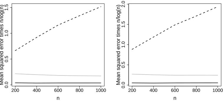
Figure 4 shows the mean (over j) of the estimated L2 PX
errors {eb(n,τj,m)}Mj=1 for
dif-ferent n, τ and m∈ {CG, P LS}. The errors were multiplied byn/log(n) to illustrate the convergence rates. According to Proposition 8 and Corollary 6 (ii) we expect the rates for the independent and autoregressive cases to ben−1log(n), which is verified by the fact that the solid black and grey lines are roughly constant. For the long range dependent case we expect worse convergence rates which are also illustrated by the divergence of the dashed black line.
6. Application to Molecular Dynamics Simulations
The collective motions of protein atoms are responsible for its biological function and molec-ular dynamics simulations is a popmolec-ular tool to explore this (Henzler-Wildman and Kern, 2007).
Typically, the p ∈ N backbone atoms of a protein are considered for the analysis with the relevant dynamics happening in time frames of nanoseconds. Although the dynamics are available exactly, the high dimensionality of the data and large number of observations can be cumbersome for regression analysis, e.g., due to the high collinearity in the columns of the covariates matrix. Many function-dynamic relationships are also non-linear (Hub and de Groot, 2009). A further complication is the fact that the motions of different backbone atoms are highly correlated, making additive non-parametric models for the target function
f∗ less suitable.
0 20 40 60 80 100
2.0
2.5
3.0
3.5
P
osition
Time in ns
0 20 40 60 80 100
0.6
0.8
1.0
1.2
1.4
1.6
1.8
Root mean square de
viation
Time in ns
Figure 5: Time series ofXt,1, i.e., the first coordinate of the first atom T4L consists of (left) and the root mean squared deviationytbetween the protein configuration at time
tand the (apo) crystal structure.
The number of available observations is n = 4601 and T4L consists of p = 486 backbone atoms.
Denote with At,i ∈R3 theith atom, i= 1, . . . , p, at time t= 1, . . . , n and ci ∈R3 the ith atom in the (apo) crystal structure of T4L. A usual representation of the protein in a regression setting is the Cartesian one, i.e., we take as the covariateXt= (AT1,t, . . . , ATp,t)T,
t= 1, . . . , n, see Brooks and Karplus (1983). The functional quantity to predict is the root mean square deviation of the protein configuration Xt at time t= 1, . . . , n from the (apo)
crystal structureC = (cT
1, . . . , cTd)
T, i.e.,
yt=
(
p−1
p
X
i=1
kXi,t−Cik2
)1/2
.
This nonlinear function was previously considered in Hub and de Groot (2009), where it was established that linear models are insufficient for the prediction.
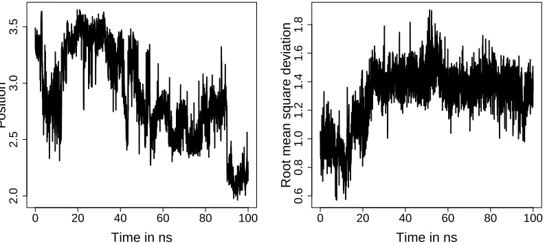
Figure 5 shows the time series corresponding toXt,1(i.e., the first coordinate of the first atom of T4L) on the left and the functional quantity yt on the right. These plots reveal
certain persistent dependence over time.
Fitting autoregressive moving average models of order (3,2) (ARM A(3,2)) to yt and
ARM A(5,2) toXt,1 shows that the smallest root of their respective characteristic polyno-mial is close to one (1.009 foryt and 1.003 forXt,1), highlighting that we are on the border of stationarity, see, e.g., Brockwell and Davis (1991).
0 20 40 60 80 100
0.75
0.80
0.85
0.90
0.95
1.00
A
utocorrelation function
Lag
0 20 40 60 80 100
0.70
0.80
0.90
1.00
A
utocorrelation function
Lag
Figure 6: Autocorrelation plots ofXt,1 (left) and yt(right). The estimated autocorrelation
function is grey, the theoretical one of a fittedARM A(3,2) process is solid black andρh∝(h+ 1)−q for a suitable choice ofq >0 is dashed black.
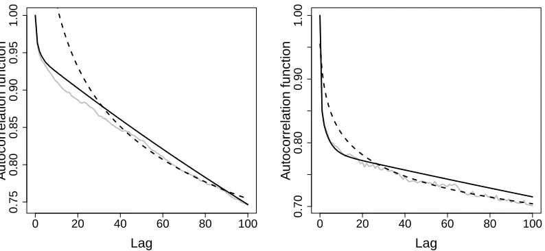
Finally, to test for long range dependence, we employed the rescaled variance test of Giraitis et al. (2003). The null hypothesis of this test is the short range dependence in the data, while the alternative is the long range dependence. Calculating the test statistics with 16 lags gives the p-value for both yt and Xt,1 smaller than 0.01, suggesting the long range dependence.
Figure 6 depicts the autocorrelation functions ofXt,1andyt, the theoretical
autocorrela-tion funcautocorrela-tion of the corresponding autoregressive moving average process andρh ∝(h+1)−q
forq= 0.134 forXt,1 andq = 0.066 foryt. The latter, as highlighted in Section 4, is an
au-tocorrelation function for a stationary long range dependent process. These plots together with the above findings suggest thatXt,1 and yt are stationary, long range dependent
pro-cesses.
We apply kernel partial least squares to this data set with the Gaussian kernelk(x, y) = exp(−lkx−yk2),x, y∈
R3p,l >0. The functionf we aim to estimate is a distance between protein configurations, so using a distance based kernel seems reasonable. Moreover, we also investigated the impact of other bounded kernels such as triangular and Epanechnikov and obtained similar results. The first 50% of the data form a training set to calculate the kernel partial least squares estimator and the remaining data are used for testing.
The parameter l > 0 is calculated via cross validation on the training set. In our evaluation we obtainedl= 10.22.
2 4 6 8 10
0.0
0.2
0.4
0.6
0.8
1.0
Correlation
Number of components
2 4 6 8 10
0.0
0.5
1.0
1.5
2.0
2.5
3.0
3.5
Correlation
Number of components
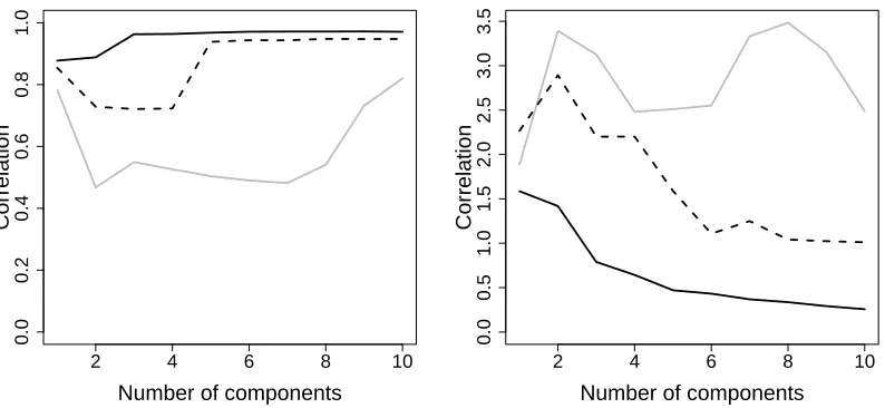
Figure 7: Correlation (left) and residual sum of squares (right) between predicted values and the observed response on the test set depending on the number of used components for kernel partial least squares (solid black), partial least squares (grey) and kernel principal component regression (dashed black).
more components. Obviously, linear partial least squares can not cope with the non-linearity of the problem.
This application highlights that kernel partial least squares still deliver a robust predic-tion even for long range dependent data, if enough observapredic-tions are available.
Acknowledgements
The authors are grateful to the action editor and two reviewers for their valuable comments which helped to improve the article. The support of the German Research Foundation via FOR 916 (Project B5) and CRC 803 (Proejct Z2) is gratefully acknowledged.
Appendix A. Source Condition and Effective Dimensionality for Gaussian Kernels
The source condition (S) and the effective dimensionality dλ are of great importance in
the convergence rates derived in Section 3. Here we investigate these conditions for the reproducing kernel Hilbert space corresponding to the Gaussian kernelk(x, y) = exp(−lkx−
yk2), x, y∈
Rd, l >0, for d= 1. Hence, the space H is the space of all analytic functions that decay exponentially fast, see Steinwart et al. (2005).
We also impose the normality conditions (D1) and (D2) on {Xt}t∈Z, where now σ2x =
Proposition 7 Assume that (K1),(K2) and (S) hold for r 1/2. Let d = 1, X0
N(0, σx2), σ2x >0 and consider the Gaussian kernel k(x, y) = exp{−l(x−y)2} for x, y∈R,
l > 0. Then f can be expressed for µ=r−1/2∈ N via f(x) = P∞
i=1ciLµ(x, zi) for fixed
{zi}∞i=1,{ci}∞i=1 ⊂R such that
P∞
i,j=1cicjk(zi, zj)≤R2, R >0. Here we have for x, z∈R Lµ(x, z) = exp
−1/2
det(Λ)(x2+z2)−2lµ+1xz
det(Λ1:µ)
,
with Λ∈R(µ+1)×(µ+1) being a tridiagonal matrix with elements
Λi,j =
σ−2x + 2l , i=j < µ+ 1
l , i=j=µ+ 1 −l , |i−j|= 1
0 , else
for i, j= 1, . . . , µ+ 1 and Λ1:µ is theµ×µ-dimensional sub-matrix ofΛ including the first
µ columns and rows.
Conversely any function f∗ = T f with f of the above form fulfills a source condition
(S) withr=µ+ 1/2, µ∈N.
Hence if we fix an r ≥ 1/2 with r−1/2 ∈ N this theorem gives us a way to construct functions f ∈ H withf∗=T f that fulfill (S).
The next proposition derives the effective dimensionality dλ in this setting:
Proposition 8 Let d = 1, X0 ∼ N(0, σx2) for some σx2 > 0 and consider the Gaussian
kernel k(x, y) = exp{−l(x−y)2},x, y∈
R,l >0.
Then there is a constant D >0 such that it holds for any λ∈(0,1]
dλ = tr{(S+λ)−1S} ≤Dlog(1 +a/λ),
with a=√2(1 +β+√1 +β)−1/2, β = 4lσx2.
With the latter result Corollary 4 is applicable and we expect convergence rates for the kernel partial least squares algorithm of order O{γnlog(1/2γn−2)} for a sequence {γn}n as
in Theorem 2.
Appendix B. Proofs
B.1 Proof of Theorem 1
The proof of Theorem 1 makes use of the connection between the partial least squares and the conjugate gradient algorithm. This section is structured as follows: First we will intro-duce the link between kernel partial least squares and kernel conjugate gradient. We will state some key facts about orthogonal polynomials and their relationship to the algorithm in Lemma 9. Then the consistency of kernel partial least squares is shown with the help of three error bounds that are obtained in Lemmas 11 — 13.
B.1.1 Orthogonal Polynomials and Some Notation
Denote with Pi the set of polynomials of degree at mosti= 0, . . . , n. For functions ψ, φ: R → R and r ∈ N0 define the inner products [ψ, φ]r = hψ(Sn)Tn∗y, Snrφ(Sn)Tn∗yiH. From the definition of the Krylov space it is immediate that every element v ∈ Ki(Sn, Tn∗y),
i= 1, . . . , n, can be represented by a polynomialq∈ Pi−1 via v=q(Sn)Tn∗y.
The following discussion is based on Hanke (1995), chapter 2. There exist two sequences of polynomials {pi}ni=0,{qi}ni=0 ⊂ Pi, such thatfi =qi−1(Sn)Tn∗y with q−1 = 0 and Tn∗y−
Snfi = pi(Sn)Tn∗y. Both sequences are connected by the equation pi(x) = 1−xqi−1(x), x∈R, and the polynomials{pi}ni=0 are orthogonal with respect to [·,·]0.
We will also consider other sequences of polynomials, namely {q[ir]}n i=0,{p
[r]
i }ni=0 ⊂ Pi,
q−1[r] = 0, such that pi[r](x) = 1−xq[i−1r] (x), x∈R, and the sequence {p[ir]}n
i=0 is orthogonal with respect to [·,·]r. This yields for every r∈N0 a separate conjugate gradient algorithm with solution fi[r] =qi[r−1] (Sn)Tn∗y ∈ Ki(Sn, Tn∗y) and residuals Tn∗y−Snfi[r] = p[ir](Sn)Tn∗y,
i= 1, . . . , n. Thep[ir],i= 0, . . . , n,r ∈N0, are called residual polynomials.
AsSnis self-adjoint, positive semi-definite and the kernel is bounded byκwe know that
its spectrum is a subset of [0, κ], see Caponnetto and de Vito (2007). This also implies that max{kSkL,kSnkL} ≤κ, withk · kLdenoting the operator norm. Theidistinct roots ofp[ir] will be denoted by 0< x[1r,i] < . . . xi,i[r]< κ,i= 1, . . . , n.
We will summarize some key facts about the orthogonal polynomials in the next lemma.
Lemma 9 Let r, s∈N0 and i= 1, . . . , n. Then we have:
(i) The roots of consecutive orthogonal polynomials interlace, i.e., forj= 1, . . . , iit holds
0< x[j,ir]+1< x[j,ir]< x[j,ir+1]< x[jr+1] ,i+1 < xj[r+1] ,i<· · ·< xi,i[r+1]< x[ir+1] ,i+1< κ,
(ii) the optimality property [p[1]i , p[1]i ]01/2=kTn∗y−Snfi[1]kH≤ kTn∗y−SnhkH holds for all
h∈ Ki(Sn, Tn∗y),
(iii) on x∈[0, x[1r,i]]it holds 0≤pi[r](x)≤1 andq[ir](x)≤
p[ir]
0
(0)
,
(iv) p[nr]=p[ns],
(v) p[ir]0(0) =−Pi
j=1
x[j,ir]−1,
(vi) for r ≥ 1 define φi(x) = p[ir](x)
x[1r,i]
1/2
x[1r,i]−x
−1/2
, x ∈ [0, x[1r,i]], i = 1, . . . , n.
Then it holds for u≥0 that xuφ2i(x)≤uu
p[ir]0(0)
−u
with the convention 00 = 1.
Proof: (i) See Hanke (1995), Corollary 2.7.
(ii) See Hanke (1995), Proposition 2.1.
Because of the convexity ofpi on [0, x1,i] we getqi (x) =x−1{1−pi (x)} ≤
pi (0) .
(iv) See the discussion in Hanke (1995) preceding Proposition 2.1 and use the facts that
Tn∗y∈range(Sn) andSn is an operator of rank n.
(v) Write p[ir](x) =Qi
j=1(1−x/x [r]
j,i), x∈[0, κ], and the result is immediate.
(vi) See equation (3.10) in Hanke (1995).
We denote for x ≥ 0 by Px the orthogonal projection operator on the eigenspace
cor-responding to the eigenvalues of Sn that are smaller or equal x and Px⊥ = IH−Px with
IH:H → H being the identity operator.
B.1.2 Preparation for the Proof
We consider the kernel partial least squares algorithm as an optimization problem
fi = arg min g∈Ki(Sn,Tn∗y)
n−1ky−Tngk2, i= 1, . . . , n. (8)
This is the conjugate gradient algorithm CGNE discussed in chapter 2.2 of Hanke (1995), to which we refer for more details. Note that, for example,
n−1hφ(TnTn∗)y, TnTn∗ψ(TnTn∗)yi=hφ(Sn)Tn∗y, ψ(Sn)Tn∗yiH= [φ, ψ]0, for polynomialsφ, ψ.
In the upcoming proofs we will make use of the following operator inequality:
Lemma 10 Let B, C : H → H be two positive semi-definite, self-adjoint operators with
max{kBkL,kCkL} ≤κ. Then it holds for any r≥0 withζ = max{r−1,0}
kBr−CrkL≤(ζ+ 1)κζkB−CkrL−ζ.
Proof: See Blanchard and Kr¨amer (2010b), Lemma A.6.
For the remainder of the proof we assume that we are on the set where it holds with probability at least 1−ν,ν∈(0,1], thatkSn−SkL≤Cδ(ν)γnandkTn∗y−SfkH≤C(ν)γn
for a sequence {γn}n converging to zero and constantsCδ=Cδ(ν), C=C(ν)>0.
With Lemma 2.4 in Hanke (1995) we see that the stopping iteration (5) can also be expressed as
a∗= minn1≤a≤n:kSnfa[1]−T
∗
nykH≤Cγn
o
, (9)
i.e., we stop the kernel partial least squares algorithm when a discrepancy principle forfa[1]
holds.
It is easy to see that from (S) it follows for r≥1/2 that
(SH) There existµ≥0,R >0 and u∈ Hsuch that f =Sµu andkukH≤R.
This condition is known as the H¨older source condition withµ=r−1/2. Recall that H ⊆ L2 PX
and T :H → L2 PX
is the change of space operator. Using the fact that T,T∗ are adjoint operators, fa∗=T fa∗ and f∗=T f forr≥1/2 we see
An application of Lemma 10 yields
kfa∗−f∗k2 =kS1/2(fa∗−f)kH≤ kS1/2(fa∗−f[1]
a∗)kH+kS1/2(fa[1]∗ −f)kH
≤Cδ1/2γn1/2
kfa∗−f[1]
a∗kH+kfa[1]∗ −fkH
+kSn1/2(fa∗−f[1]
a∗)kH+kSn1/2(fa[1]∗ −f)kH. (10)
The following lemmas will deal with bounding the quantities in (10) in terms of the source parameter r = µ+ 1/2 ≥ 1/2 and the sequence γn. First we will derive upper
bounds for the quantities containing the difference of the KPLS estimator fa∗ and the
estimator fa[1]∗:
Lemma 11 Assume Cx ∈ (0,1] such that x∗ = (Cxγn)1/(µ+1) < x[1]1,a∗−1 and C > C+
CxR+Cδ(µ+ 1)κµR. Under the conditions of the theorem it holds µ≥0
kfa∗−f[1]
a∗kH≤γnµ/(µ+1)
C
Cx1/(µ+1)[1−C−1{C+CxR+Cδ(µ+ 1)κµR}]2
kSn1/2(fa∗−f[1]
a∗)kH≤γn(2µ+1)/(2µ+2)
C
Cx1/(2µ+2)[1−C−1{C+CxR+Cδ(µ+ 1)κµR}]
.
Proof: If the inner products [·,·]0 and [·,·]1 are the same the proof is done because both
polynomial sequences are identical.
We now observe that we have for a∗ = n due to Lemma 9 (iv) qn−1(x)−q[1]n−1(x) = x−1{p[1]n (x)−pn(x)}= 0, i.e., kfa∗−fa[1]∗kH= 0 and kSn1/2(fa∗−fa[1]∗)kH= 0 and the proof is done.
If the inner products differ and we have 0< a∗ < nit holds fa∗ 6=f[1] a∗.
Proposition 2.8 in Hanke (1995) can now be applied for 0< a∗ < nand yieldsqa∗−1(x)−
qa[1]∗−1(x) =x−1{p
[1]
a∗(x)−pa∗(x)}=θa∗p[2]
a∗−1(x),x≥0, withθa∗ = (p[1]
a∗)0(0)−(p
[0]
a∗)0(0)>0.
We getfa∗−f[1]
a∗ =qa∗−1(Sn)T∗ ny−q
[1]
a∗−1(Sn)Tn∗y=θa∗p[2]
a∗−1(Sn)Tn∗y.
Proposition 2.9 in Hanke (1995) yieldsθa∗ =
h
p[2]a∗−1, p
[2]
a∗−1
i−1
1 h
p[1]a∗, p
[1]
a∗
i
0. The optimal-ity property offa[1]∗ in Lemma 9 (ii) shows that
kTn∗y−Snfa[1]∗kH=kp[1]a∗(Sn)Tn∗ykH= h
p[1]a∗, p[1]a∗
i1/2
0
≤hp[2]a∗−1, p[2]a∗−1
i1/2
0 . (11)
Combining these results yields
kfa∗−f[1] a∗kH=
h
p[1]a∗, p
[1]
a∗
i
0 h
p[2]a∗−1, p
[2]
a∗−1
i
1 h
p[2]a∗−1, p
[2]
a∗−1
i1/2
0 ≤
h
p[2]a∗−1, p
[2]
a∗−1
i
0 h
p[2]a∗−1, p
[2]
a∗−1
i
1
Recall thatx1,a∗−1 denotes the first root ofpa∗−1. It holds for any 0≤x≤x1,a∗−1 that
0≤p[2]a∗−1(x)≤1, see Lemma 9 (iii), and thus
h
p[2]a∗−1, p
[2]
a∗−1
i1/2
0 ≤ kPxp [2]
a∗−1(Sn){Tn∗y−Sf+Sf}kH+kPx⊥p
[2]
a∗−1(Sn)Tn∗ykH
≤Cγn+kPxp[2]a∗−1(Sn)Sµ+1ukH+x−1/2kPx⊥Sn1/2p
[2]
a∗−1(Sn)Tn∗ykH
≤Cγn+xµ+1R+kPxp
[2]
a∗−1(Sµ+1−Snµ+1)ukH+ 1 √
x
h
p[2]a∗−1, p
[2]
a∗−1
i1/2
1 . In the second inequality (SH) withµ≥0 was applied.
By assumption x∗ = (Cxγ)1/(µ+1)≤x
[1]
1,a∗−1< x
[2]
1,a∗−1 due to the interlacing property of
the roots of the polynomialsp[ir],i= 1, . . . , n,r ∈N0, see Lemma 9 (i).
Using Lemma 10 we get kSµ+1−Snµ+1kL≤(µ+ 1)κµCδγn and setting x=x∗ we get h
p[2]a∗−1, p
[2]
a∗−1
i1/2
0 ≤Cγn+x
µ+1
∗ R+Cδγn(µ+ 1)κµR+x
−1/2 ∗
h
p[2]a∗−1, p
[2]
a∗−1
i1/2
1 =γn{C+CxR+Cδ(µ+ 1)κµR}+x
−1/2 ∗
h
p[2]a∗−1, p[2]a∗−1
i1/2
1 . (13) Due to (9) and (11) we have additionally Cγn≤ kSnfa[1]∗−1−Tn∗ykH=kp[1]a∗−1(Sn)Tn∗ykH≤ h
p[2]a∗−1, p
[2]
a∗−1
i1/2
0 .
Plugging this into (13) yields
h
p[2]a∗−1, p
[2]
a∗−1
i1/2
0 ≤
C+CxR+Cδ(µ+ 1)κµR
C
h
p[2]a∗−1, p
[2]
a∗−1
i1/2
0 + 1 √
x∗ h
p[2]a∗−1, p
[2]
a∗−1
i1/2
1 , or equivalently withx∗= (Cxγn)1/(µ+1)
h
p[2]a∗−1, p
[2]
a∗−1
i1/2
0 ≤γ
−1/(2µ+2)
n
h
p[2]a∗−1, p
[2]
a∗−1
i1/2
1
Cx1/(2µ+2)[1−C−1{C+CxR+Cδ(µ+ 1)κµR}]
, (14)
where by assumption C > C+CxR+Cδ(µ+ 1)κµR and x∗ = (Cxγ)1/(µ+1).
Combining (12), (14) and kp[1]a∗(Sn)Tn∗ykH≤Cγn due to the stopping index (9) yields
kfa∗−f[1]
a∗kH≤γn−1/(µ+1)
kp[1]a∗(Sn)Tn∗ykH
Cx1/(µ+1)[1−C−1{C+CxR+Cδ(µ+ 1)κµR}]2
≤γnµ/(µ+1) C
Cx1/(µ+1)[1−C−1{C+CxR+Cδ(µ+ 1)κµR}]2
.
For the second part of the proof we derive in the same way as (12)
kSn1/2(fa∗−f[1] a∗)kH≤
h
p[2]a∗−1, p
[2]
a∗−1
i1/2
0 h
p[2]a∗−1, p
[2]
a∗−1
i1/2
1
Using (14) andkp[1]a∗(Sn)Tn∗ykH≤Cγn gives
kSn1/2(fa∗−f[1]
a∗)kH≤γn(2µ+1)/(2µ+2)
C
Cx1/(2µ+2)[1−C−1{C+CxR+Cδ(µ+ 1)κµR}]
,
finishing the proof.
We now derive an upper bound on the quantities that containfa[1]∗ andf. These contain
kSnfi[1] −Tn∗ykH, which can be controlled for i=a∗ by the discrepancy principle (9), and
(p[1]i )0(0), for which we have to derive a separate bound later on.
Lemma 12 For anyi= 1, . . . , nand any 0< x≤x[1]1,i we have under the conditions of the
theorem for µ≥1
kf−fi[1]kH≤Rxµ+Cδµκµ−1γn +x−1
n
kSnfi[1]−T
∗
nykH+ (C+CδκµR)γn
o
+ (C+CδκµR)γn|(p[1]i )
0(0)|,
kSn1/2(f−fi[1])kH≤R n
xµ+1/2+x1/2Cδµκµ−1γn
o
+x−1/2
n
kSnfi[1]−Tn∗ykH+ (C+CδκµR)γn
o
+x1/2(C+CδκµR)γn|(p[1]i )0(0)|.
Proof: Denote ¯fi=q[1]i−1(Sn)Snf and consider
kf −fi[1]kH≤ kPx(f−f¯i)kH+kPx( ¯fi−fi[1])kH+kP
⊥
x (f−f
[1]
i )kH. (15)
The first term of (15) can be bound by an application of Lemma 10 and (SH) withµ≥1
kPx(f −f¯i)kH=kPx{I−q[1]i−1(Sn)Sn}fkH=kPxp[1]i (Sn)fkH =kPxp[1]i (Sn)SµukH ≤ kPxp[1]i (Sn)SnµukH+kPxp[1]i (Sn)(Sµ−Snµ)ukH
≤Rxµ+Cδµκµ−1γn .
In the last inequality we used that on 0≤x≤x[1]1,i we have 0≤p[1]i (x)≤1.
For the second term of (15) we use Lemma 9 (iii) qi[1](x) ≤ |(p[1]i )0(0)| on x ∈ [0, x[1]1,i]. This yields
kPx(fi[1]−f¯i)kH =kPxq[1]i (Sn)(Snf−Tn∗y)kH
≤ kPxq[1]i (Sn)(Sf−Tn∗y)kH+kPxqi[1](Sn)(Sn−S)fkH ≤(C+CδκµR)γn
p[1]i 0(0)
.
Finally, we have
kPx⊥(f −fi[1])kH≤x−1kPx⊥Sn(f−fi[1])kH ≤x−1
n
kSnfi[1]−Tn∗ykH+kPx(Tn∗y−Snf)kH o
≤x−1nkSnfi[1]−T
∗
nykH+ (C+CδκµR)γn
and thus the first inequality is proven. For the second inequality we use
kSn1/2(f−fi[1])kH≤ kPxSn1/2(f−f¯i)kH+kPxSn1/2( ¯fi−fi[1])kH+kP
⊥
x Sn1/2(f −f
[1]
i )kH.
In the same way as before we derive bounds for the three terms:
kPxSn1/2(f −f¯i)kH≤x1/2Cδµκµ−1Rγn+xµ+1/2R,
kPxSn1/2( ¯fi−fi[1])kH≤x1/2(C+CδRκµ)γn
p[1]i
0 (0) ,
kPx⊥Sn1/2(f−fi[1])kH≤x−1/2{kSnfi[1]−Tn∗ykH+ (C+CδκµR)γn},
completing the proof.
Lemma 12 depends on (p[1]i )0(0) and hence an upper bound for this term is needed: Lemma 13 Assume that Cx ∈ (0,1] is such that x∗ = (Cxγ)1/(µ+1) < x[1]1,a∗−1 and C >
C+CxR+Cδ(µ+ 1)κµR. Under the conditions of the theorem it holds for µ≥0
p[1]a∗
0 (0)
≤γn−1/(µ+1)
"
Cx−1/(µ+1)
1−C+CxR+Cδ(µ+ 1)κ
µR
C
−2
+
(2µ+ 2)µ+1R C−Cδ(µ+ 1)κµR+C
1/(µ+1)#
Proof: The proof is done in two steps by using the inequality
p[1]a∗
0 (0) ≤
p[1]a∗−1
0 (0) +
p[1]a∗
0
(0)−p[1]a∗−1
0 (0) .
Consider firsta∗ >1.
We will boundkSnfa[1]∗−1−Tn∗ykHfrom above. Definez=x[1]1,a∗−1 andφi(x) =p[1]i (x)(z−
x)−1/2z1/2, 0 ≤ x ≤ z. Due to Lemma 9 (vi) it holds that sup0≤x≤zxνφ2a∗−1(x) ≤
νν|(p[1]a∗−1)0(0)|−ν,ν ≥0. The proof of Lemma 3.7 in Hanke (1995) shows that
h
p[1]a∗−1, p
[1]
a∗−1
i1/2
0 ≤ kPzφa
∗−1(Sn)Tn∗ykH.
This yields with (SH)
kSnfa[1]∗−1−Tn∗ykH= h
p[1]a∗−1, p
[1]
a∗−1
i1/2
0 ≤ kPzφa
∗−1(Sn)Tn∗ykH
≤ kPzφa∗−1(Sn)SfkH+kPzφa∗−1(Sn)(T∗
ny−Sf)kH
≤ kPzφa∗−1(Sn)SfkH+Cγn
sup 0≤x≤z
φ2a∗−1
1/2
≤ kPzφa∗−1(Sn)Sµ+1
n ukH+kPzφa∗−1(Sn)(Sµ+1
n −Sµ+1)ukH+Cγn
≤R
(
sup 0≤x≤z
x2µ+2φ2a∗−1
1/2
+Cδ(µ+ 1)κµγn
sup 0≤x≤z
φ2a∗−1
1/2)
+Cγn
≤
p[1]a∗−1
0 (0)
−µ−1
This gives together withCγn≤ kSnfa[1]∗−1−Tn∗ykH Cγn≤
p[1]a∗−1
0 (0)
−µ−1
(2µ+ 2)µ+1R+{Cδ(µ+ 1)κµR+C}γn.
IfC > Cδ(µ+ 1)κµR+C we finally have
p[1]a∗−1
0 (0)
≤γn−1/(µ+1)
(2µ+ 2)µ+1R C−Cδ(µ+ 1)κµR+C
1/(µ+1)
. (16)
If a∗ = 1 it holds p[1]a∗−1 = 1 and thus
p[1]a∗−1
0 (0)
= 0 and the inequality (16) is true as
well.
We will derive an upper bound on
p[1]a∗
0
(0)−p[1]a∗−1
0 (0)
.Due to Corollary 2.6 of
Hanke (1995) we have
p[1]a∗−1
0
(0)−p[1]a∗
0 (0) ≤ h
p[1]a∗−1, p
[1]
a∗−1
i
0 h
p[2]a∗−1, p
[2]
a∗−1
i
1
. (17)
We have 0≤x≤x[1]1,a∗−1 < x[2]1,a∗−1 due to the interlacing property of the roots in Lemma
9 (i) and thus 0≤p[2]a∗−1(x)≤1 for 0≤x≤x[2]1,a∗−1. With that we get with (SH)
kp[1]a∗−1(Sn)Tn∗ykH≤ h
p[2]a∗−1, p
[2]
a∗−1
i1/2
0
≤ kPxp[2]a∗−1(Sn)Tn∗ykH+x−1/2kPx⊥S1n/2p[2]a∗−1(Sn)Tn∗ykH
≤ kPxp[2]a∗−1(Sn)(Tn∗y−Sf)kH+kPxp[2]a∗−1(Sn)Sµ+1ukH+x−1/2 h
p[2]a∗−1, p
[2]
a∗−1
i1/2
1 ≤Cγn+R
Cδ(µ+ 1)κµγn+xµ+1 +x−1/2
h
p[2]a∗−1, p[2]a∗−1
i1/2
1 . For the choicex∗= (Cxγ)1/(µ+1) we get
h
p[1]a∗−1, p[1]a∗−1
i1/2
0
≤γn{C+Cδ(µ+ 1)κµR+Cx}+x
−1/2 ∗
h
p[2]a∗−1, p[2]a∗−1
i1/2
1 . It holdshp[1]a∗−1, p[1]a∗−1
i1/2
0 =
kSnfa[1]∗−1−Tn∗ykH ≥Cγn. This yields with C > C+CxR+
Cδ(µ+ 1)κµR
h
p[1]a∗−1, p[1]a∗−1
i
0
≤γn−1/(µ+1)Cx−1/(µ+1)
1−C+CxR+Cδ(µ+ 1)κ
µR
C
−2
h
p[2]a∗−1, p[2]a∗−1
i
1. Together with (17) we have
p[1]a∗−1
0
(0)−p[1]a∗
0 (0)
≤γn−1/(µ+1)Cx−1/(µ+1)
1−C+CxR+Cδ(µ+ 1)κ
µR
C
−2
.
B.1.3 Proof of Theorem 1
The proof is an application of Lemmas 11 — 13 to (10). First note that r ≥3/2 implies
µ≥1 and thus this condition in Lemma 12 holds.
Let us choose x∗ = (Cxγn)1/(µ+1). Lemma 9 (v) shows that
p[ir] 0
(0)
=Pi j=1(x
[r]
j,i)−1
fori= 1, . . . , n,r∈N0. Thus it holds
p[1]i
0
(0)
−1
≤x[1]1,i.
Equation (16) thus shows that Cx can be chosen small enough such that
x∗≤
p[1]a∗−1
0
(0)
−1
≤x[1]1,a∗−1
and Cx <1, which makes the first condition in Lemma 11 and 13 hold true. The choice
C=C+ (µ+ 1)κµR(1 +Cδ) gives the second condition.
Now we need to check the remaining condition of Lemma 12, namely that a Cz can
be chosen such that (Czγn)1/(µ+1) ≤ x[1]1,a∗ is true. Lemma 13 yields a Cz > 0 such that
Czγn1/(µ+1) ≤
p[1]a∗
0
(0)
−1
≤ x[1]1,a∗. Denote z∗ = (Czγn)1/(µ+1) and Lemma 12 can be
applied.
To ease notation we will denote everything in the derived bounds that does not depend on γn as a constant cj, j ∈ N. Thus we get by combining Lemmas 12 and 13 that with probability at least 1−ν
kf−fa[1]∗kH2 ≤c1γnµ/(µ+1)+c2γn+c3γn1−1/(µ+1)+c4γn
p[1]a∗
0
(0)
≤c1γnµ/(µ+1)+c2γn+c3γnµ/(µ+1)+c5γn1−1/(µ+1) =O{γnµ/(µ+1)}
and
kSn1/2(f −fa[1]∗)k2H
≤c6γn(µ+1/2)/(µ+1)+c7γn1/(2µ+2)γn+c8γn−1/(2µ+2)γn+c9γn1/(2µ+1)γn
p[1]a∗
0
(0)
≤c6γn(µ+1/2)/(µ+1)+c7γn(2µ+3)/(2µ+2)+c8γn(2µ+1)/(2µ+2)+c10γn1+1/(2µ+2)−1/(µ+1)
=O{γn(2µ+1)/(2µ+2)}.
Finally Lemma 11 gives
kfa∗−f[1]
a∗k2H =O{γnµ/(µ+1)}, kSn1/2(fa∗−f[1]
a∗)kH=O{γn(2µ+1)/(2µ+2)}.
Combining the above with (10) yields
kf −fa∗kH2 =O{γµ/(µ+1)
n },
kf∗−fa∗k22=O{γ1/2γnµ/(µ+1)}+O{γn(2µ+1)/(2µ+2)}=O{γn(2µ+1)/(2µ+2)},
B.2 Proof of Theorem 2
The overall design of this proof is similar to the one of Theorem 1 and makes heavy use of results obtained in Blanchard and Kr¨amer (2010b).
B.2.1 Preparation for the Proof
The stopping index (7) can be reformulated with µ=r−1/2 as
a∗= min{1≤a≤n:kSnfa[1]−Tn∗ykH≤Cζn}, (18)
withζn= max{
√
λndλγn, λµn+1}.
We will derive the result in a similar way to Theorem 1. First it holds due to (10)
kfa∗−f∗k2 =kS1/2(fa∗−f)kH≤ kS1/2(fa∗−f[1]
a∗)kH+kS1/2(fa[1]∗ −f)kH ≤Cψλ1/2kfa∗−f[1]
a∗kH+CψkSn1/2(fa∗−f[1]
a∗)kH+kS1/2(fa[1]∗ −f)kH. (19)
Now we prove the analogue versions of Lemma 11 — 13. The comments regarding those lemmas also hold here.
Lemma 14 Let x = Cxλn, Cx > 0 such that 0 < x < x[2]1,a∗−1. Choose C > ˜c2, with
˜
c1 =Rmax{1, Cψ2, µκµ−1Cδ} and ˜c2 = 2 max{CψC
√
Cx+ 1,˜c1Cx(Cxµ+ 1)}. Then it holds
kfa∗−f[1] a∗kH ≤
C3 Cx(C−c˜2)2
λ−1n ζn,
kSn1/2(fa∗−f[1] a∗)kH ≤
C2 Cx1/2(C−˜c2)
λ−1n /2ζn.
Proof: According to the proof of Lemma 14 we can focus on the case 0< a∗ < n. Further-more we have due to (12)
kfa∗−f[1] a∗kH ≤
h
p[2]a∗−1, p
[2]
a∗−1
i
0 h
p[2]a∗−1, p[2]a∗−1
i
1
kp[1]a∗(Sn)Tn∗ykH. (20)
Using Lemma A.3 in Blanchard and Kr¨amer (2010b) (and the first line of its proof) we have for 0< x < x[2]1,a∗−1 with ˜c1 =Rmax{1, Cψ2, µκµ−1Cδ}
h
p[2]a∗−1, p
[2]
a∗−1
i1/2
0 ≤CψC p
x+λn
p
dλnγn+ ˜c1x{xµ+Zµ(λn)}+x−1/2
h
p[2]a∗−1, p
[2]
a∗−1
i1/2
1 . (21)
Choosing x=Cxλn yields in (21)
h
p[2]a∗−1, p
[2]
a∗−1
i1/2
0 ≤CψC
p
Cx+ 1
p
λndλnγn+ ˜c1Cx(Cxµ+ 1)λµn+1+Cx−1/2λ−1n /2
h
p[2]a∗−1, p
[2]
a∗−1
i1/2
1 ≤˜c2max{
p
λndλnγn, λµn+1}+C
−1/2
x λ
−1/2
n
h
p[2]a∗−1, p[2]a∗−1
i1/2
1 = ˜c2ζn+Cx−1/2λ
−1/2
n
h
p[2]a∗−1, p
[2]
a∗−1
i1/2
1 , with ˜c2 = 2 max{CψC
√
Cx+ 1,˜c1Cx(Cxµ+1)}. Due to the stopping condition (18) we know
that
h
p[2]a∗−1, p[2]a∗−1
i1/2
0
≥hp[1]a∗−1, p[1]a∗−1
i1/2
0 =
kSnfa[1]−Tn∗ykH≥Cζn.
This gives
h
p[2]a∗−1, p
[2]
a∗−1
i1/2
0 ≤
C
√
Cx(C−c˜2) λ−1n /2
h
p[2]a∗−1, p
[2]
a∗−1
i1/2
1 . (22)
Plugging this into (20) yields together with the definition of the stopping indexa∗
kfa∗−f[1] a∗kH≤
C3 Cx(C−˜c2)2
λ−1n ζn.
In a similar way we derive for the second case
kSn1/2(fa∗−f[1] a∗)kH=
h
p[1]a∗, p
[1]
a∗
i
0 h
p[2]a∗−1, p
[2]
a∗−1
i1/2
1 ≤
h
p[2]a∗−1, p
[2]
a∗−1
i1/2
0 h
p[2]a∗−1, p
[2]
a∗−1
i1/2
1 h
p[1]a∗, p[1]a∗
i
0.
An application of (22) yields
kSn1/2(fa∗−f[1] a∗)kH≤
C2
√
Cx(C−˜c2)
λ−1n /2ζn.
Lemma 15 Denote ˜c1 = Rmax{1, Cψ2, µκµ−1Cδ}. For any i= 1, . . . , n and 0 < x < x[1]1,i we have under the conditions of the theorem
kS1/2(fi[1]−f)kH≤Cψ
Cδ+
√
2C+λn
Cδ
p[1]i
0 (0) + √
2Cx−1
p
dλnγn
+ ˜c1( √
x+pλn)(xµ+λµn) + (1 +
p
x−1λn)x−1/2kSnfi[1]−Tn∗ykH. Proof: Follow the proof of Lemma A.2 in Blanchard and Kr¨amer (2010b). Note that
![Figure 1: The function f evaluated on [−7.5, 7.5] (black) and one realisation of the noisydata y = f(x) + ε (grey).](https://thumb-us.123doks.com/thumbv2/123dok_us/9787881.1964386/11.612.202.403.112.302/figure-function-evaluated-black-realisation-noisydata-e-grey.webp)