© 2017 IJSRSET | Volume 3 | Issue 6 | Print ISSN: 2395-1990 | Online ISSN : 2394-4099 Themed Section: Engineering and Technology
Modified Quick Switching Variables Sampling System Indexed
by Six Sigma Quality Levels
Dr. D. Senthilkumar, B. Esha Raffie
Department of Statistics, PSG College of Arts & Science, Coimbatore, Tamilnadu, India
ABSTRACT
This paper is an attempt of modified quick switching variables sampling system indexed by six sigma quality levels [QSVSS-r (nσ; kT, kN), r=2 and 3]. This plan gives operating and designing procedures of the sampling system.
Those procedures verified with practical applications and also constructed tables for easy selection of plans given indexed by six sigma quality levels.
Keywords: Modified Quick Switching Variables Sampling System, Operating Characteristic Curve, Six Sigma AQL and Six Sigma LQL.
I.
INTRODUCTION
Six Sigma was developed as a set of rules to improve and maintain the manufacturing processes and may avoid defects, but its application was subsequently extended to all area of business processes as well. In Six Sigma, a defect is defined as anything that could lead to customer dissatisfaction. The particulars of the methodology were first formulated by Bill Smith at Motorola in 1986. Six Sigma was heavily inspired by six preceding decades of quality improvement methodologies such as quality control, TQM, and Zero Defects, based on the work of pioneers such as Shewhart, Deming, Juran, Ishikawa, Taguchi and others. In acceptance sampling plan major area occupied by Quick switching system, Quick switching system was originally proposed by Dodge (1967) and investigated by Romboski (1969). Romboski (1969) has made a brief study of the modified quick switching systems, namely QSS-r (nσ; cN, cT), r = 2 and 3. Romboski (1969) has
studied the QSS-1 by taking a single sampling plan as reference plan. Based on this study, he has made some modification to the switching rules of QSS. The modified systems are designated as QSS-2 and QSS-3. Soundararajan and Arumainayagam (1989) have studied the properties of these modified systems and observed the advantages, and Soundararajan and Arumainayagam (1990) have provided tables for the selection of QSS for various given conditions. Since the single sampling QSS-r(n, kn; c0), r = 2 and 3 system has more than two
parameters, a variety of plans can be found satisfying the given (AQL, LQL) condition. The modified systems result in a composite OC curve, which is more discriminating one than the original QSS-1. These are more efficient than QSS-1. Palanivel (1999) has studied modified quick switching system designing procedures applied in variables sampling plan for given a combination of (AQL, LQL). Senthilkumar and Esha Raffie (2012) have studied six sigma quick switching variable sampling system (nσ; kT, kN) constructed by
(SSAQL, 1-) and (SSLQL, β), where =3.4 x 10⁻⁶ and
β ≥ 2, six sigma quality levels. In later Senthilkumar and Esha Raffie (2015) have studied six sigma quick switching variable sampling system (nTσ, nNσ; kσ) for
given six sigma quality levels of SSAQL and SSLQL for tighten sample size. Senthilkumar and Esha Raffie (2016) have constructed six sigma modified quick switching variables sampling system [SSMQSVSS-r ( nTσ, nNσ; kσ), r=2 and 3] indexed by six sigma quality
levels of SSAQL and SSLQL.
In this paper, tables and procedures for selection of QSVSS-r (nσ; kT, kN), r=2 and 3 indexed by Six Sigma
AQL, α (producer’s risk), Six Sigma LQL, β (Consumer’s risk) is indicated. This QSVSS-r (nσ; kT, kN), r=2 and 3 is
constructed with a point on the OC curve (SSAQL, 1-)
and (SSLQL, β), where =3.4 x 10⁻⁶ and β ≥ 2 is similar
1. Six Sigma Modified Quick Switching Variables Sampling System [SSQSVSS-r(nσ; kT, kN), r=2
and 3]
The conditions and the assumptions under which the
SSMQSVSS can be applied are as follows:
The production is steady, so that results on current and preceding lots are broadly indicative of a continuous process.
Lots are submitted substantially in the order of production.
Inspection is by variables, with the quality being defined as the fraction of non- conforming.
The sample units are selected from a large lot and production is continuous.
The production process depends on automation and human involvement in the process is negligible. The industry may adopt system method with
decision makers have an experience in adopting the six sigma quality initiatives.
Basic Assumptions
The quality characteristic is represented by a random variable X measurable on a continuous scale.
Distribution of X is normal with mean and standard deviation.
An upper limit U, has been specified and a product is qualified as defective when X>U. [when the lower limit L is Specified, the product is a defective one if X<L].
The Purpose of inspection is to control the fraction defective, p in the lot inspected.
When the conditions listed above are satisfied the fraction defective in a lot will be defined by
p= 1-F(v)=F(-v)with p and
2/2
1 F(y)
2
z
e dz
y
(1)
where z ~ N (0, 1). Here the decision criterion for the σ- method variables plan is to accept the lot if ̅ σ
where U is the upper specification limit or if ̅ σ where L is the lower specification limit.
2. SSQSVSS-r((nσ; kTσ, kNσ), where r=2 and 3)
with known σ for given SSAQL and SSLQL
The Six Sigma Modified Quick Switching Variables Sampling System with known σ variables plan as the reference plan has the following Operating Procedure
Operating Procedure
Step 1: Draw a sample of size nσ from the lot through
normal inspection, inspect and record the measurement of the quality characteristic for each unit of the sample. Compute the sample
mean
X.
Step 2: If ̅ σσ or ̅ σσ accept the
lot and repeat Step 1 otherwise, go to Step 3.
Step 3: Under tightened inspection, draw a sample of size nσ from the next lot inspect and
record the measurement of the quality characteristic for each unit of the sample.
Compute the sample mean
X.
Step 4: If ̅ σσ or ̅ σσ accept the
lot. When r consecutive lots are accepted, switch to Step 1, otherwise repeat Step 3.
where kNσand kTσare the acceptance criterion of the variable sampling plan under normal and tightened inspection respectively. Tightened inspection may be achieved by reducing kN but leaving nσ fixed. This
moves the OC curve to the left, thus reducing the consumer’s risk but increasing the producer’s risk. Under σ-method X and σ are the average quality characteristic and standard deviation respectively.
3. Operating Characteristic Function
Romboski (1969) derived the OC function of the QSS-r(n, cN, cT), r=2 and 3. Based on this, the OC function of
SSQSVSS-2(nσ; kTσ, kNσ) and SSQSVSS-3(nσ; kTσ, kNσ)
are respectively given by
The OC function of SSQSVSS-2(nσ; kTσ, kNσ) is
2
N T T N T
a 2
T N T
P P +P (1-P )(1+P ) P (p)=
P +(1-P )(1+P ) (2)
The OC function of SSQSVSS-3(nσ; kTσ, kNσ) is
3 2
N T T N T T
a 3 2
T N T T
P P +P (1-P )(P +P +1) P (p)=
where PT and PN are the proportion of lots expected to
be accepted using tightened (n, kT) and normal (n, kN)
variable single sampling plans respectively.
Under the assumption of normal approximation to the non-central t distribution (Abramowitz and Stegun, 1964), the values of PN and PT are given b
N N N
P =F(w )pr[(U-X) / σk ] (4)
T T T
P =F(w )pr[(U-X) / σk ] (5) where
T σ T T σ
w = n (U-k σ-μ)/σ=(v-k ) n
N σ N N σ
w = n (U-k σ-μ)/σ=(v-k ) n
and
ν = (U -μ) / σ
4. Designing SSQSVSS-r(nσ; kTσ, kNσ), r=2 and 3
Satisfying Pa(p1) ≥ 1-α and Pa(p2) ≤ β
In view of the properties of SSAQL and SSLQL discussed in Section 1 of the Chapter V, p1 and p2 are
used as the reference quality levels defined as Pa(p1) ≥ 1-α
Pa(p2) ≤ β
Table 1 and 2 give the values of nσ, kN, and kT the
given values of p1, p2, α and β.
5. Selection of SSQSVSS-r(nσ; kTσ, kNσ), r=2 and 3
with known σ for given SSAQL and SSLQL
For SSMQSVSS-2(nσ; kTσ, kNσ), to determine the values
of nσ, kTσ, and kNσ the given values of p1, p2, α and β
should satisfy the following equations.
1 1 1 1 1
1 1 1
2
N T T N T
a 1 2
T N T
P P +P (1-P )(1+P )
P (p )= 1 α
P +(1-P )(1+P ) (6)
2 2 2 2 2
2 2 2
2
N T T N T
a 2 2
T N T
P P +P (1-P )(1+P )
P (p )= β
P +(1-P )(1+P ) (7) For SSQSVSS-3(nσ; kTσ, kNσ), to determine the values of
nσ, kTσ, and kNσ the given values of p1, p2, α and β
should satisfy the following
equations.
1 1 1 1 1 1
1 1 1 1
3 2
N T T N T T
a 1 3 2
T N T T
P P +P (1-P )(P +P +1)
P (p )= 1 α
P +(1-P )(P +P +1) (8) 2 2 2 2 2 2
2 2 2 2
3 2
N T T N T T
a 2 3 2
T N T T
P P +P (1-P )(P +P +1)
P (p )= β
P +(1-P )(P +P +1)
(9)
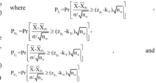
where 1
1 1
p
T p T σ
σ
X-X
P =Pr (z -k ) n
σ/ n
,
1
1 1
p
N p N σ
σ X-X
P =Pr (z -k ) n σ/ n
,
2
2 2
p
T p T σ
σ
X-X
P =Pr (z -k ) n
σ/ n
, and
2
2 2
p
N p N σ
σ X-X
P =Pr (z -k ) n
σ/ n
z is standard normal variate, zp1 and zp2 are standard
normal variates at p1 and p2 respectively.
For given SSAQL and SSLQL, the parametric values of SSQSVSS-r namely kT, kN and the sample size nσ are
determined by using a computer search C++ programme.
6. Designing SSQSVSS-r(nσ; kTσ, kNσ), r=2 and 3
with known σ for given SSAQL and SSLQL
Example
Table 1 can be used to determine SSQSVSS-2(nσ; kTσ,
kNσ) for specified values of SSAQL and SSLQL. For
example, if it is desired to have a SSQSVSS-2(nσ; kTσ,
kNσ) for given SSAQL = 0.000005 and SSLQL =
0.00006, α= 3.4x10⁻⁶, β ≥ 2α. Table 1 gives n = 1426, kT = 3.25, kN = 2.965 as desired system parameters,
which is associated with 4.4 sigma level.
Practical Application
For the test, lot-by-lot acceptance inspection of compact disc it is proposed to apply the system with n=1426, kT=3.250 and kN=2.965. The characteristic to be
inspected is the compact disc with the upper limit (U) diameter of 120 mm with a known standard deviation (σ) of 0.05 mm.
Now, take a random sample of size n=1426 and record the diameter of each compact disc. Compute the sample mean (X). If X+kN σ ≤ U ⇒ X+ (2.965) (0.05) ≤ 120,
accept the lot. Otherwise, switch to tightened inspection. Draw a sample of 1426 from the next lot and record the results. Compute the sample mean (X). If X+kT σ ≤ U
consecutive lots are accepted, then switch to normal inspection. Otherwise, continue with tightened inspection process.
Example
Table 2 can be used to determine SSQSVSS-3(nσ; kTσ,
kNσ) for specified values of SSAQL and SSLQL. For
example, if it is desired to have a SSQSVSS-3(nσ; kTσ,
kNσ) for given SSAQL = 0.000002 and SSLQL =
0.000003, α= 3.4x10⁻⁶
, β ≥ 2α. Table 2 gives n = 7145,
kT = 4.413, kN = 4.371 as desired system parameters,
which is associated with 4.7 sigma level.
Practical Application
For the test, lot-by-lot acceptance inspection of globe bulb it is proposed to apply the system with n=7145, kT=4.413 and kN=4.371. The characteristic to be
inspected is the globe bulb with the upper limit (U) length of 5 inches with a known standard deviation (σ) of 0.006 inches.
Now, a random sample of size n=7145 is taken and the length of each globe bulb recorded. Compute the sample mean (X). If X+kN σ ≤ U ⇒ X+(4.371) (0.006) ≤ 5,
accept the lot. Otherwise, switch to tightened inspection. Draw a sample of 7145 from the next lot and record the results. Compute the sample mean (X). If X+kT σ ≤ U
⇒ X +(4.413) (0.006) ≤ 5, accept the lot. When 3 consecutive lots are accepted, then switch to normal inspection. Otherwise, continue with tightened inspection process.
7. Selection of SSQSVSS-r(nS; kTS, kNS), where r=2
and 3, with unknown σ for given SSAQL and SSLQL
The steps involved in this procedure are as follows Step 1: Draw a sample of size ns from the lot, inspect
and record the measurement of the quality characteristic for each unit of the sample. Compute the sample mean X and sample standard deviation S.
Step 2: If ̅ or ̅ accept the lot and repeat Step 1 otherwise go to Step 3. Step 3: Draw a sample of size ns from the next lot
inspect and record the measurement of
the quality characteristic for each unit of the sample. Compute the sample mean X sample standard deviation S.
Step 4: If ̅ or ̅ accept the lot. When r consecutive lots are accepted, switch to Step 1, otherwise repeat Step 3.
where X and S are the average and the standard deviation of quality characteristic respectively from the sample. Under the assumptions for a Six Sigma Quick Switching System stated, the probability of acceptance Pa(p) of a lot is SSQSVSS-2 and SSQSVSS-3 are given
by (2) and (3) and PT and PN respectively are
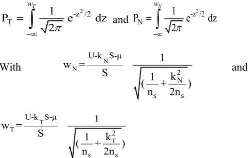
2
-z /2
T 1
P e dz
2 T
w
and PN 1 e-z /22 dz2 N
w
With N N 2
N
s s
U-k S-μ 1
w =
S 1 k
( + )
n 2n
and
T T
T
2
s s
S
U-k -μ 1
w =
S 1 k
( + )
n 2n
For SSQSVSS-2(nS; kTS, kNS), to determine the values
of nS, kT , and kN the given values of p1, p2, α and β
should satisfy the following equations.
1 1 1 1 1
1 1 1
2
N T T N T
a 1 2
T N T
P P +P (1-P )(1+P )
P (p )= 1 α
P +(1-P )(1+P ) (10)
2 2 2 2 2
2 2 2
2
N T T N T
a 2 2
T N T
P P +P (1-P )(1+P )
P (p )= β
P +(1-P )(1+P ) (11)
For SSQSVSS-3(nS; kTS, kNS), to determine the values
of nS, kT and kN the given values of p1, p2, α and β
should satisfy the following equations.
1 1 1 1 1 1
1 1 1 1
3 2
N T T N T T
a 1 3 2
T N T T
P P +P (1-P )(P +P +1)
P (p )= 1 α
P +(1-P )(P +P +1) (12)
2 2 2 2 2 2
2 2 2 2
3 2
N T T N T T
a 2 3 2
T N T T
P P +P (1-P )(P +P +1)
P (p )= β
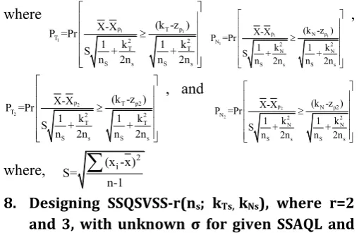
where
1 1
1
p T p
T 2 2
T T
S s S s
(k -z ) X-X
P =Pr
k k
1 1
S + +
n 2n n 2n
1 1
1
p N p
N 2 2
N N
S s S s
(k -z ) X-X
P =Pr
k k
1 1
S + +
n 2n n 2n
,
2 2
p T p2
T 2 2
T T
S s S s
(k -z ) X-X
P =Pr
k k
1 1
S + +
n 2n n 2n
, and
2 2
p N p2
N 2 2
N N
S s S s
(k -z ) X-X
P =Pr
k k
1 1
S + +
n 2n n 2n
where, (x -x)i 2 S=
n-1
8. Designing SSQSVSS-r(ns; kTs, kNs), where r=2
and 3, with unknown σ for given SSAQL and SSLQL
Example
Table 1 can be used to determine SSQSVSS-2 (ns; kTs,
kNs) for specified values of SSAQL and SSLQL. For
example, if it is desired to have a SSQSVSS-2(ns; kTs,
kNs) for given SSAQL= 0.0001 and SSLQL =0.0007,
α= 3.4x10⁻⁶
, β ≥ 2α. Table 1 gives n = 13587, kT =
2.152, kN = 1.890 as desired system parameters, which
is associated with 5.1 sigma level.
Practical Application
For the test, lot-by-lot acceptance inspection of an electrical switch control knob it is proposed to apply the system with n=13587, kT=2.152 and kN=1.890. The
characteristic to be inspected is an electrical switch control knob with the upper limit (U) diameter of 1.31 inches.
Now, take a random sample of size n=13587 and record the diameter of each electrical switch control knob. Compute the sample mean (X) and unknown standard deviation (S). If X+kN S ≤ U ⇒ X+ (1.890) S ≤ 1.31,
accept the lot. Otherwise, switch to tightened inspection. Draw a sample of 13587 from the next lot and record the results. Compute the sample mean ( X ) and unknown standard deviation (S). If X+kT S ≤ U ⇒ X
+(2.152) S ≤ 1.31, accept the lot. When 2 consecutive lots are accepted, then switch to normal inspection. Otherwise, continue with tightened inspection process.
Example
Table 2 can be used to determine SSQSVSS-3(ns; kTs,
kNs) for specified values of SSAQL and SSLQL. For
example, if it is desired to have a SSQSVSS-3(ns; kTs,
kNs) for given SSAQL = 0.00001 and SSLQL =0.00003,
α= 3.4x10⁻⁶
, β ≥ 2α. Table 2 gives n = 14141, kT =
3.446, kN = 3.321 as desired system parameters, which
is associated with 5.0 sigma level.
Practical Application
For the test, lot-by-lot acceptance inspection of Fountain Pen it is proposed to apply the system with n=14141, kT=3.446 and kN=3.321. The characteristic to be
inspected is the Fountain Pen with the upper limit (U) weightof 27 grams.
Now, take a random sample of size n=14141, record the weightof each Fountain Pen. Compute the sample mean (X) and unknown standard deviation (S). If X+kN S ≤
U ⇒ X+ (3.321) S ≤ 27, accept the lot. Otherwise, switch to tightened inspection.
Draw a sample of 14141 from the next lot and record the results. Compute the sample mean ( X ) and unknown standard deviation (S). If X+kT S ≤ U ⇒ X
+(3.446) S ≤ 27, accept the lot. When 3 consecutive lots are accepted, then switch to normal inspection. Otherwise, continue with tightened inspection process.
9. Construction of Table 1 and 2
The OC function of SSQSVSS-r(nσ; kTσ, kNσ), r=2 and 3,
is given by Equation (2) and (3). Under assumption of the normal model, the OC function of SSQSVSS-2 is given Equation (6) and (7) are solved for n, kT and kN
(known σ) for a specified pair of points, say, p1, p2, αand
β on the OC Curve. Under assumption of the normal model, the OC function of SSQSVSS-3 is given Equation (8) and (9) are solved for n, kT and kN (known
σ) for as specified pair of points, say, p1, p2, αand β on
the OC Curve. The values of nσ, kTσ, kNσ, ns, kTs and kNs
are obtained by using computer search routine through C++ programme.
Table 1 and Table 2 provided the values of nσ, kTσ, kNσ,
ns, kTs and kNs which satisfying the Equations (6), (7), (8)
and (9). The sigma (σ) value is calculated using the process sigma calculator for given n, kT and kN for
II.
CONCLUSION
In this paper an attempt is made to design of MQSVSS which has the quality of acceptance 1-3.4 x 10⁻⁶ in the
long run. This system will help the industrial production engineers, to use total quality control practices, of which the sampling inspection system is an approach used for manufacturing products. Tables are provided here which tailor-made, handy and ready-made use to the industrial shop-floor condition. If this quality levels SSAQL and SSLQL are known, these system are most suitable for auto machine Company and who are applying Six Sigma initiative in their organization.
III.
REFERENCES
[1]. Abramowitz, M. and Stegun, I. A. (1964): Handbook of Mathematical Functions, National bureau of Standards, Applied Mathematical Series No. 55. [2]. Dodge, H.F. (1967): A New Dual System of
Acceptance Sampling Technical Report No.16, The Statistics Center, Rutgers – The State University , New Brunswick, NJ.
[3]. Palanivel, M. (1999): Contribution to the study Designing of Quick Switching Variables System and Other Plans, Ph.D thesis, Bharathiar University, Coimbatore, Tamil Nadu.
[4]. Romboski, L. D. (1969): An Investigation of Quick Switching Acceptance Sampling Systems. Doctoral Dissertation, Rutgers the State University, New Brunswick, New Jersey.
[5]. Soundararajan, V. and Arumainayagam, S. D. (1989): An Examination of Some Switching Procedures Used in Sampling Inspection, International Journal of Quality & Reliability Management, Vol. 6 No.5, pp
[6]. Soundararajan, V. and Arumainayagam, S. D. (1990): Construction and Selection of Modified Quick Switching System, Journal of Applied Statistics, Vol.13, No.1, pp 83-114.
[7]. Senthilkumar, D. and Esha Raffie, B. (2012): Six Sigma Quick Switching Variables Sampling System Indexed by Six Sigma Quality Levels, International Journal of Computer Science & Engineering Technology (IJCSET), Vol. Vol. 3 No. 12, pp.565-576.