2013
Improvements to random forest methodology
Ruo Xu
Iowa State University
Follow this and additional works at:
https://lib.dr.iastate.edu/etd
Part of the
Statistics and Probability Commons
This Dissertation is brought to you for free and open access by the Iowa State University Capstones, Theses and Dissertations at Iowa State University Digital Repository. It has been accepted for inclusion in Graduate Theses and Dissertations by an authorized administrator of Iowa State University Digital Repository. For more information, please [email protected].
Recommended Citation
Xu, Ruo, "Improvements to random forest methodology" (2013).Graduate Theses and Dissertations. 13052. https://lib.dr.iastate.edu/etd/13052
by
Ruo Xu
A dissertation submitted to the graduate faculty
in partial fulfillment of the requirements for the degree of
DOCTOR OF PHILOSOPHY
Major: Statistics
Program of Study Committee:
Dan Nettleton
Daniel J. Nordman, Major Professor
Stephen B. Vardeman
Kenneth Koehler
Huaiqing Wu
Iowa State University
Ames, Iowa
2013
TABLE OF CONTENTS
ABSTRACT
...
iv
CHAPTER 1: GENERAL INTRODUCTION
... 1
1
Introduction
... 1
2 Section Organization
... 1
3 Introduction to Classification and Regression Tree
... 2
4 Introduction to Random Forests and Extensions ... 6
5 Properties of Random Forests
... 8
6 Random Forest Variations
... 11
CHAPTER 2: PREDICTOR AUGMENTATION IN RANDOM FORESTS
... 16
1 Introduction
... 18
2 Improved Predictions via Data Augmentation with Independent Explainatory Variables
... 20
3 Improvement by Variable Augmentation in Real Data Examples
... 27
4 Other Considerations Impacting the Effect of Variable Augmentation
... 28
5 Conclusions and Qualifications
... 32
CHAPTER 3: ITERATIVE BIAS CORRECTION IN RANDOM FORESTS
... 36
1 Introduction
... 36
2 Bias Correction for Random Forests
... 38
3 Real Data Examples
... 41
4 Generalization of Bias Correction in Random Forests
... 42
5 Conclusion
... 44
CHAPTER 4: CASE-SPECIFIC RANDOM FORESTS
... 48
1 Introduction
... 50
2 Case-specific Random Forests by Weighted Bootstrap
... 51
3 Simulation and Real Data Examples
... 53
4 Case-Specific Variable Importance
... 55
5 Data Illustration
... 58
6 Conclusions
... 59
CHAPTER 5: CASE-SPECIFIC ESTIMATION OF EXPECTED PREDICTION LOSS
... 66
1 Introduction
... 66
2 Estimation of Case-Specific Expected Prediction Loss
... 68
3 Simulation Studies
... 71
4 Discussion
... 74
GENERAL CONCLUSIONS
... 82
ABSTRACT
Random forest (RF) is a widely used machine learning method that shows competitive prediction performance in various fields, including biological science, finance, chemical engineering, agroscience, medical analysis, etc. In this dissertation, we study some characteristics and modifications of RFs in order to improve its prediction performance.
In CHAPTER 1, we review the mechanics of classification and regression trees (CARTs), bootstrap aggregation (bagging) and RFs. The properties of RFs are discussed, along with several variations of this method.
In CHAPTER 2, we describe a counter-intuitive discovery using RFs: the out-of-sample prediction errors can be reduced by augmenting the regressor with a new scientifically meaningless predictor variable independent of all variables in the dataset. We explain this phenomenon using a simulated example and discuss the importance of this result in interpreting predictor variable importance in RFs.
RF predictions can be biased. In CHAPTER 3, we apply an iterative debiasing approach based on bagging to RFs and test this bias correction method with real datasets. The debiasing approach can significantly improve RF predictions. The number of debiasing iterations can be tuned using cross-validation.
Standard RF methodology generates a common RF from a given training sample, regardless of test cases. In CHAPTER 4, we propose a new way to grow a RF specifically predicting a particular test case, namely, Case-Specific Random Forests (CSRF). We also suggest Case-Specific Variable Importance (CSVI), a new definition of predictor variable importance in terms of the prediction performance on a particular test case.
Prediction error estimation is generally useful in evaluation of a prediction rule. All present methods deal with estimating prediction errors averaging over the distribution of a test set. In CHAPTER 5, we propose a method to estimate expected prediction loss on a specific regressor point using RF methodology.
CHAPTER 1. GENERAL INTRODUCTION
1
Introduction
Random forest (RF) methodology is a machine learning technique useful for prediction problems. The RF algorithm, developed by Leo Breiman (2001a), applies bootstrap aggregation (bagging) (Breiman 1996a,b) and random feature selection (Ho 1995, 1998; Amit and Geman 1997) to individual classification or regression trees for prediction. There are many studies showing that RFs have impressive predictive performance in regression and classification problems in various fields, including financial forecasting, remote sensing, and genetic and biomedical analysis (Siroky 2009; Kumar and Thenmozhi 2006; Shi et al. 2005; Ward et al. 2006; Diaz-Uriarte and de AndršŠs 2006; Jiang et al. 2007; Pal 2003; Palmer et al. 2007; Goldstein et al. 2011). The RF method has been compared with other learning methods, such as partial least squares regression, support vector machine and neural networks in Breiman (2001a), Kumar and Thenmozhi (2006), Diaz-Uriate and Alvarez de Andrez (2006), and Palmer et al. (2007). In such comparisons, RFs typically shows comparable or even better prediction performance. Besides
the appealing prediction performance by RFs, the availability of computation package randomForest in
R (Liaw and Wiener 2002) is another reason for its great popularity. To date, Breiman’s original paper (2001a) has been cited over 3700 times according to Web of Science. A good resource for using RFs is Leo Breiman’s website http://www.stat.berkeley.edu/~breiman/RandomForests/cc_home.htm.
2
Section Organization
In this thesis, we study properties of random forests and the approaches to improve the prediction performance by RFs as outlined in the thesis abstract. In order to present modifications for improving RFs and understand the exposition to follow, it is first helpful to provide an overview of the basic mechanics and properties of RFs, which we seek to do in this chapter.
A RF is an ensemble of tree predictors, with each independently and randomly generated tree depend-ing on the values of a random vector (Breiman 2001a). To appreciate the RF algorithm, it is initially helpful to understand the mechanism of growing a single decision tree. In Section 3, we will introduce how a single tree is generated. In Section 4, we describe the algorithm of growing a RF, which includes a series of randomly generated trees. In Section 5, we discuss various byproducts of RFs, such as the proximity measure and measure of predictor variable importance, which are important in later chapters for developing modifications and improvements to RFs. We also discuss how a RF deals with predictor
variables with missing values. In Section 6, we introduce some useful extensions of the RF method.
3
Introduction to Classification and Regression Tree
Classification and Regression Trees (CARTs) belong to the family of binary tree structured regressors or classifiers (Breiman et al. 1984). Understanding how a CART is generated is critical in order to understand how a RF works. Thus, we first review the mechanism of CARTs. Most of the material is adopted from (Breiman et al. 1984). The algorithm-based approach for creating a CART involves repeated binary splits of sets of objects, namely nodes or leaves, into two descendant subsets (called subnodes or subleaves). For each split, one predictor variable and a corresponding “cut-point” (chosen according to some within-subnode homogeneity criterion described in Subsection 3.2) are used to partition a node into two subnodes.
3.1
Ways to Deal with Different Predictor Types
If a predictor variable xj is numerical, the candidate cut-points are the unique midpoints of the
intervals between ordered values from this predictor (from the available cases in a given node). Then
node cases are partitioned into two subnodes depending on whether the value ofxj is below or above the
cut-point. For example, suppose in a nodeS containing five cases, the values ofxj are -1.0, 1.0, 1.0, 2.8
and 3.6. Then the corresponding unique midpoints are 0, 1.9 and 3.2. So three possible binary splits by
xj are “ifxj >0or not”, “if xj >1.9or not” and “if xj >3.2or not”. We see it is the order of xj values
but not their actual values that matters.
If a predictor variablexj is categorical without ordinality, dummy variables need to be made. For an
xj with Gcategorical levels in nodeS, there will be2G−1−1possible binary splits. For example, if the
cases in a nodeS have the three unique categories,red, blue and green, then we can split node S onxj
in three ways, “ifred or not”, “ifblueor not” and “ifgreen or not”.
3.2
Grow a Tree Iteratively by Measuring Node Heterogeneity
The fundamental idea of node splitting is to make each subnode as homogeneous as possible after the current splitting. Hence CART is a greedy method. The function for heterogeneity measure must be a concave function, so that the function quantity will never increase after any split (Coppersmith et al.
1999). Denote the parent node to be split asS, and the left and right subnodes asLandR. For regression
IS =
X
i∈S
(yi−y¯)2, (1)
wherey¯is the average of response values in nodeS. Then the decrease of heterogeneity of nodeS after
splitting intoLandR is
∆I(S, L, R) = IS−(IL+IR). (2)
For classification trees, the Gini index of diversity or entropy is often used to reflect the impurity of
a node S. Suppose there are G categories in the data. With πS(g) defined as the proportion of the
observations from thegth category in nodeS, and nS as the number of cases in nodeS, the Gini index
is defined as nS· G X g=1 πS(g) [1−πS(g)], (3)
and the entropy is defined as
nS· G
X
g=1
πS(g) [−log(πS(g))]. (4)
TakingIS to be either (3) or (4), the decrease of impurity of nodeS after split is defined by (2) as in the
regression case. In the standard CART approach, the chosen split for each node is the one that maximizes ∆I(S, L, R)in (2). This process is repeated until a largest possible tree is obtained and no more nodes
can be split.
3.3
Prediction by a Tree
Once a tree is grown, we need to assign a predicted value for each terminal node. Suppose a terminal
nodeNodek contains nk training casesC1, . . . , Cnk with Ci ≡(xi, yi), then the prediction for a given
ˆ yk = 1 Pnk i=1wi nk X i=1 wi·yi, (5)
wherewi, i= 1, . . . , nk are nonnegative numbers. In regression problems,
wi = 1 nk . In classification problems, wi = 1 if Pnk l=1I(yl=yi)≥ Pnk l=1I(yl=yj)∀yi6=yj, 0 otherwise,
whereI(·)denotes the indicator function. This means the prediction for a regression problem is simply
the arithmetic average of all training case responses inNodek, while that for classification is the category
receiving a plurality of votes by all training cases in the node.
Because a CART is a way to partition the regressor space to disjoint hyperrectangles, a test case with
given predictor values will end up in one terminal node. All test cases falling in a terminal nodeNodek
will be predicted usingyˆk in (5).
3.4
Pruning a Tree
Usually the largest treeTmax, in which there are no more splits that can be done, performs badly for
prediction of a new test dataset, because the variance of prediction increases as the size of the tree exceeds
the optimal. Accordingly, pruning is conducted to avoid this overfitting problem. For a treeT withK
terminal nodes, let R(T) denote the overall training sample error of this tree. Let α be a complexity
parameter, which quantifies the penalty for increasing the size of the tree by splitting one node. Define
the cost-complexity measure of treeT as
Rα(T) = R(T) +αK. (6)
define T(α) to be the tree that minimizes Rα(T) over all trees T that are subtrees of Tmax (i.e., trees
that can be further split to obtainTmax). T(α)has the following properties: i)T(α)is a subtree ofTmax;
ii)T(α)yields the least cost-complexity measure Rαamong all the subtrees ofTmax; iii)T(α)yields the
least training errorRamong all the subtrees ofTmaxcontaining same number of terminal nodes T(α).
Asα increases, the minimizing treeT(α) has fewer terminal nodes. The largest tree Tmax has only
a finite number of subtrees. Hence if T(α) is the minimizing tree for some α, it continues to be the
minimizing tree asα increases until a jump point α0 is reached, although the complexity parameterα
is a positive continuous number. For example, it could be that some treeTa is the minimizing tree for
α∈(0.1,0.2], and another smaller tree Tb is minimizing forα∈(0.2, 0.25]. It can be proved that the
sequence of minimizing trees{Tj(αj), j= 1, 2, . . .}is a nested tree sequence, which means thatTp(αp)is a
subtree ofTq(αq)forαp> αq. This nested sequence characteristic makes the pruning process computation
feasible. Instead of checking all the subtrees ofTmax which can be an extremely large number, we only
need to look at this nested sequence of minimizing trees.
What value should αtake? The goal of pruning is to select a tree from{Tj(αj), j = 1,2, . . .} that
gives the lowestout-of-sampleprediction error for an independent dataset. Cross-validation is a preferred
method for this purpose. For aV-fold cross-validation, the training sample is randomly separated intoV
subsets, each containing the same or nearly the same number of elements. Letsubsetv denote thevth of
theV subsets. Letsamplevdenote the training sample obtained by combining all subsets exceptsubsetv.
In a V-fold cross-validation, the largest possible tree is grown for each of the V training samples,
sample1, . . . , sampleV. Let Tmax, v denote the largest tree grown for samplev, v = 1, . . . , V. From
Tmax, v, the nested minimizing tree sequence{Tj(αj), j= 1,2, . . .} can be obtained, andsubsetv serves
as an independent test sample for each minimizing treeTj, v(αj). An prediction error RCV(α) for allV
minimizing trees can be calculated as a function ofα. The optimal complexity parameterαCV corresponds
to the size of the tree producing the lowestRCV(α).
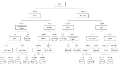
Once a CART is pruned, a prediction value is assigned to each terminal node as explained in Subsection 3.3. An example of classification tree with two categories is adopted from Hammann et al. 2010 and is shown in Figure 1.
Figure 1: An example of a classification tree.
4
Introduction to Random Forests and Extensions
4.1
Bootstrap Aggregation (Bagging)
A large decision tree may lead to large prediction variance. Pruning alleviates overfitting, but it was Breiman’s bootstrap aggregation method (bagging, Breiman 1996a; Buhlmann and Yu 2002; Friedman and Hall 2000) that effectively solved the overfitting problem. Bagging is an ensemble learning method. Other ensemble methods include boosting, stacking, and bumping (Freund and Schapire 1996; Hastie
et al. 2009). Bagging has been shown able to effectively reduce prediction variance forunstableprediction
rules. The terminstability was explained heuristically by (Breiman 1996b) and then more systematically
defined by (Buhlmann and Yu 2002), according to whom, a statisticθˆn is called stable if
ˆ
θn → θasn→ ∞,
for some fixed valueθ, where θis not necessarily E(ˆθn). Buhlmann and Yu (2002) argued that unstable
prediction rules arise mainly when hard-thresholding decisions with indicators are involved. A decision tree is nothing but partitioning the regressor space with disjoint hyper-rectangles. The prediction by a decision tree is a weighted average of all responses from a terminal node (Subsection 3.3). Therefore the predicted value for some new case can be written in the form of a step function,
ˆ
By Buhlmann and Yu’s definition (2002), a CART is not a stable prediction rule. By averaging results from bootstrap resamples, bagging smoothes the response surface and hence reduce the prediction variance.
Suppose we have a training setC={C1, . . . , Cn}, then the bagging algorithm is as follows,
1) TakeM bootstrap resamples of C, sayB1, . . . ,BM.
2) For each resampleBm,m= 1, . . . M, fit the model as done for the original training data C to obtain
ˆ
fm∗, the fitted prediction rule that maps the predictor space to the response space.
3) Then the prediction for a new caseC0 with covariatex0 is
1 M
PM
m=1fˆm∗(x0) for regression problems
and
argmaxg{PMm=1I[ ˆfm∗(x0) =g]} for classification problems.
4.2
Random Subspace Method
Two factors affect the prediction errors of an ensemble of trees: (1) how accurate the individual trees are, and (2) how dissimilar the trees are from each other. Factor 1 is responsible for prediction bias by the whole forest of trees, while factor 2 is related to prediction variance of the forest. The bagging approach avoids generating exactly the same trees by resampling with replacement, which in turn reduces prediction variance and alleviates overfitting by the tree ensemble. Apart from this, there are other ways to create dissimilar trees.
Ho (1995; 1998) and Amit and Geman (1997) independently proposed to grow trees only on a randomly chosen subspace, instead of the whole regressor space. The authors showed that the combined tree classifier grown using random subspaces was better than individual trees in terms of prediction errors. There are many ways to apply the random subspace method in decision trees, including randomly choosing a subset of predictors at the tree level or at the split level, randomly choosing a subset of cut-points for a predictor variable before splitting, etc. Geurts et al. (2006) proposed extremely randomized trees, where splits (both predictor variable and its cut-points) are selected completely at random. Many machine learning methods balance the “bias-variance trade-off,” so that a satisfactory prediction error can be obtained. Similarly RFs uses the bagging approach and the random subspace idea to substantially smooth prediction and reduce prediction variance, without sacrificing prediction accuracy too much. When a split is to be made, only
a subset of predictor variables are randomly selected and considered as split candidates. Our experience shows that a random selection of predictors at the split level is better than a selection at the tree level.
4.3
The Random Forest Algorithm
Now we are ready to describe the RF algorithm. Suppose we have a training setC ={C1, . . . , Cn}
withCi≡(xi, yi)and an independent test caseC0 with predictorx0.
1) Sample the training setCwith replacement to generate bootstrap resamplesB1, . . . ,BM.
2) For each resample Bm, m = 1, . . . , M, grow a classification or regression tree Tm as described in
Section 3, except for the following modifications.
a) At each split, only predictors in a randomly selected subset of predictors are considered as discussed
in Section 4.2. Letpdenote the total number of predictor variables inC.Breiman suggested usingbp/3c
as this number, which is the default set up in the R packagerandomForest.
b) Each tree is grown until all nodes contain observations no more than themaximal terminal nodesize,
MTN, a pre-specified parameter. Unlike CART, trees in RFs are not pruned.
3) For predicting the test caseC0with covariatex0, the predicted value by the whole RF is obtained by
combining the results given by individual trees. Letfˆm∗(x0)denote the prediction ofC0bymth tree, the
RF prediction is 1 M PM m=1fˆ ∗
m(x0) for regression problems
argmaxg{P M
m=1I[ ˆfm∗(x0) =g]} for classification problems.
(7)
5
Properties of Random Forests
5.1
Tuning Random Forests
Breiman (2001a) first argued that the number of trees in a forest is a complexity parameter and tried to prove that overfitting could be overcome by growing more trees. However, it is the maximal terminal nodesize (MTN) not the number of trees that is a complexity parameter of RFs. A RF is fundamentally
an adaptivek-nearest neighbor predictor (Lin and Jeon 2006). For a single decision tree, the MTN value
specifies thek value corresponding to the k-nearest neighbor method, which controls the complexity of
the decision tree. Growing an ensemble of trees makes the prediction function (7) smoother than that of an individual tree, but the MTN value still controls the depth of each tree, and in turn controls the
complexity of the whole forest. In the R packagerandomForest, the default MTN value is 5 for regression
bootstrap-based error estimation techniques.
5.2
Out-of-bag Predictions
Cross-validation and bootstrap are two major techniques to non-parametrically estimate prediction error for a given model or statistical method (Borra and Ciaccio 2010; Hastie et al. 2009). When the size
of a training sampleC is not small, a bootstrap resampleCmalmost always contains only a subset of the
original sample. Therefore the model fitted byCm,fˆm∗, can be used to predict the cases inC\Cm, and
a prediction error estimate is obtained by averaging the out-of-sample errors on all training cases (Efron 2004, Efron and Tibshirani 1997).
A RF is generated with bootstrap samples of the training set, which naturally enables the
implemen-tation of the error estimation based on bootstrap. In the RF literature, the predictions ofC\Cm byfˆm
are calledout-of-bag (OOB) predictions, and the prediction error estimate is calledout-of-bag prediction
error. These two quantities are formally defined as follows,
1) DrawB bootstrap resamples of the training setC, namelyCm, m = 1, . . . , M. Grow a tree by Cm,
denoted asTm.
2) For any training caseCi ∈C, denote Oi as the set of indices of trees which contain contain Ci. Let
O−i beC\Oi.
3) The OOB predicted value forCi with covariatexi is
˜ yiOOB = 1 ||O−i|| X m∈O−i ˆ fm∗(xi),
where||O−i|| is the size of setO−i.
4) If we use a loss functionL(·), the OOB prediction error is
g ErrOOB = 1 n n X i=1 L(yi,y˜OOBi ).
In the R packagerandomForest, the OOB prediction and OOB prediction errors (mean squared error
5.3
Proximity Measure
As previously mentioned, RFs belong tok-nearest neighbor predictor (Lin and Jeon 2006). The tree
splitting algorithm tends to gather similar cases together in a node because each split always maximizes the decrease of heterogeneity in response values. So it is reasonable to consider cases in the same terminal nodes of a tree to be closer in proximity to each other than cases that lie in different terminal nodes. Then the relative frequency of this coincidence over all trees provides a measure of proximity between any pair of cases. The proximity measure in RF literature is defined as follows,
1) A RF ofM trees is generated on a training setC of sizen.
2) Putall training cases (Oi∪O−i) down each tree. If casesCi andCj are in the same terminal node,
thenUm ij = 1; otherwiseUijm= 0. 3) LetUij = M1 PM m=1U m
ij. Then the proximity forC based on this RF is a symetric n×nmatrix P,
with itsith row andjth column entry equal to Uij, which is the proximity between Ci andCj.
This proximity matrix is provided by the R packagerandomForest.
5.4
Predictor Variable Importance
There is no universally accepted criterion of predictor variable importance. One natural notion is that a predictor variable is important if prediction performance can be improved by using the predictor and diminished by ignoring it (Olshen 2010, pp. 1644). In Chapter 2 we will show this definition can be misleading.
Breiman proposed another way to define variable importance (Breiman 2001b) as follows. For a tree, if randomly permuting the values of a certain predictor variable for cases not included in tree construction harms the prediction for those cases, then this variable is deemed important. The variable importance defined in this way assigns highest values to variables with the greatest discrepancy between original prediction performance and prediction performance after permutation. The resulting variable importance values have no meaning on an absolute scale, but their relative sizes can be useful for comparing across different predictor variables. In regression problems, such prediction performance is computed by first tree-wise determining squared errors for predicting training cases left-out of the resampled tree construction and then averaging all such errors over all trees in the forest. In classification problems, increase in misclassification error after permutation can be taken as the measure of variable importance. This notion
5.5
Predictor Variables with Missing Values
Breiman suggested two ways of imputing missing values in predictor variables when using RFs for
prediction (see Breiman’s homepage). Notationally, suppose thejth predictor from caseCi,xij is missing.
For classification problems, ifXjis a numerical variable, a simple approach is to replace this missing value
with the median of all availablejth predictor values from cases with observed classyi. IfXjis a categorical
predictor variable, replace the missing value with the most frequent category observed in all cases with
non-missing values of the predictor and observed classyi.
Missing values in regression problems (those with quantitative response variable) is easier to deal with than classification problems. A simple imputation approach is to replace the missing value with the
median of all availablejth predictor values from the training setC, regardless of their response values.
A more complicated iterative method is as follows.
1) Use the simpler approach described above to obtain starting values for missing observations.
2) Grow a RF based on the imputed training set, and calculate all pairwise proximity measures as discussed in Section 5.3.
3) The missing value on jth predictor for Ci, xij, is replaced with a weighted average of non-missing
values based on proximity measuresMik, k ∈ Qj, where Qj is the subset of the training set whose jth
predictor values are not missing, i.e.,
˜ xij = P k∈QjMik·xkj P k∈QjMik .
4) Repeat steps 2 and 3 iteratively.
The second imputation method is more computationally intensive but provides better prediction
per-formance. Both methods are available in the R packagerandomForest.
6
Random Forest Variations
Since the invention of Breiman’s RF methodology, several variations on random forests have been developed, including random survival forests (RSF, Ishwaran et al. 2008), multivariate random forests (De’ath; Segal and Xiao 2011), enriched random forests (Amaratunga et al. 2008), quantile regression forests (Meinshausen 2006), etc. These methods either deal with different problem contexts, or were proposed with different resampling or response surface fitting mechanisms, which all contribute to the generalization of RF methodology.
6.1
Random Survival Forests
Standard RFs cannot deal with survival data with censoring. Ishwaran et al. proposed growing
decision trees with bootstrap resamples based on a splitting rule maximizing the logrank statistic after splits (Ishwaran et al. 2008). Survival functions are estimated non-parametrically in terminal nodes. The
authors also provided their computation tool in R, calledrandomSurvivalForest. In this package, they
used the Nelson-Aalen method to estimate survival functions.
6.2
Multivariate Random Forests
De’ath (2010) considered using the idea of decision trees to handle regression problems with multi-variate responses. Instead of measuring the sum of squared errors (SSEs) before and after splits on one response, the author used the sum of the SSEs from multivariate responses as the measure of node het-erogeneity. Therefore, the chosen split is the one giving the maximal decrease in the sum of SSEs. The computation tool was provided by the same author. Segal and Xiao (2011) further proposed growing an ensemble of these multivariate regression trees.
6.3
Enriched Random Forests
When the number of predictors is huge yet the number of informative predictors is relatively very small, the classification performance by RF declines dramatically because a RF randomly selects a subset of features as splitting candidates at each split. This situation can be met, for example, in microarray analyses that typically involve thousands of genes whose expression levels serve as predictor variables. Amaratunga et al. (2008) suggested evaluating how informative each predictor variable is using some
pre-filtering methods, such ast-tests, in order to roughly calculate how well a predictor can separate two
classes. Then the random selection of predictor variables is replaced by weighted selection based on the pre-filtering procedure. Thus, the chance of selecting informative variables is largely increased.
6.4
Quantile Regression Forests
RFs take the average of predictions by individual trees as the predicted value by the forest.
Mein-shausen (2006) argued that a RF actually contains the estimated distribution of FY|x(y|X0 =x), not
only the meanE(Y |X0=x). In RFs, only the averages of responses in terminal nodes are recorded in
a tree. In contrast, quantile regression forests save all training case indices in terminal nodes. Note that the predicted value by a RF is nothing but a weighted average of the training sample responses. The
the indicator function andYi is the response of training caseCi. Consistency of this estimator was proven
under certain assumptions.
References
Amaratunga, D., Cabrera, J., and Lee, Y.-S. (2008). Enriched random forests. Bioinformatics,
24(18):2010–2014.
Amit, Y. and Geman, D. (1997). Shape quantization and recognition with randomized trees. Neural
Computation, 9(7):1545–1588.
Borra, S. and Ciaccio, A. D. (2010). Measuring the prediction error. a comparison of cross-validation,
bootstrap and covariance penalty methods.Computational Statistics and Data Analysis, 54:2976–2989.
Breiman, L. (1996a). Bagging predictors. Machine Learning, 26(2):123–140.
Breiman, L. (1996b). Heuristics of instability and stabilization in model selection.The Annals of Statistics,
24(6):2350–2383.
Breiman, L. (2001a). Random forests. Machine Learning, 45:5–32.
Breiman, L. (2001b). Statistical modeling: The two cultures (with rejoinder). Statistical Science,
16(3):199–231.
Breiman, L., Friedman, J., Stone, C., and Olshen, R. (1984). Classification and Regression Trees.
Chap-man and Hall, 1st edition edition.
Buhlmann, P. and Yu, B. (2002). Analyzing bagging. Annals of Statistics, 30(4):927–961.
Coppersmith, D., Hong, S., and Hosking, J. (1999). Partitioning nominal attributes in decision trees. Data Mining and Knowledge Discovery, 3:197–217.
De’ath, G. mvpart: Multivariate partitioning, 1.3-1. R Package Version.
Diaz-Uriarte, R. and de AndršŠs, S. A. (2006). Gene selection and classification of microarray data using
random forest. BMC Bioinformatics, 7:3–15.
Efron, B. (2004). The estimation of prediction error: Covariance penalties and cross-validation. Journal
Efron, B. and Tibshirani, R. (1997). Improvements on cross-validation: The .632+ bootstrap method. Journal of the American Statistical Association, 92(438):548–555.
Freund, Y. and Schapire, R. (1996). Experiments with a new boosting algorithm. Machine Learning:
Proceedings of the Thirteenth International Conference, pages 148–156.
Friedman, J. and Hall, P. (2000). On bagging and nonlinear estimation. Journal of Statistical Planning
and Inference, 137(3):669–683.
Geurts, P., Ernst, D., and Wehenkel, L. (2006). Extremely randomized trees.Machine Learning, 63:3–42.
Goldstein, B., Polley, E., and Briggs, F. (2011). Random forests for genetic association studies.Statistical
Applications in Genetics and Molecular Biology, 10(1):1–34.
Hammann, F., Gutmann, H., Vogt, N., Helma, C., and Drewe, J. (2010). Prediction of adverse drug
reactions using decision tree modeling. Clinical Pharmacology and Therapeutics, 88:52–59.
Hastie, T., Tibshirani, R., and Friedman, J. (2009). The Elements of Statistical Learning: Data Mining,
Inference, and Prediction. Springer, 2nd edition edition.
Ho, T. (1995). Random decision forest. Proceedings of the 3rd International Conference on Document
Analysis and Recognition, Montreal, QC, 14-16:278–282.
Ho, T. (1998). The random subspace method for constructing decision forests. IEEE Transactions on
Pattern Analysis and Machine Intelligence, 20(8):832–844.
Ishwaran, H., Kogalur, U., Blackstone, E., and Lauer, M. (2008). Random survival forests. The Annals
of Applied Statistics, 2(3):841–860.
Jiang, P., Wu, H., Wang, W., Ma, W., Sun, X., and Lu, Z. (2007). Mipred: classification of real and
pseudo microrna precursors using random forest prediction model with combined features. Nucleic
Acids Research, 35(2):339–344.
Kumar, M. and Thenmozhi, M. (2006). Forecasting stock index movement: A comparison of support
vector machines and random forest.Indian Institute of Capital Markets 9th Capital Markets Conference.
Liaw, A. and Wiener, M. (2002). Classification and regression by randomforest. R News, 2(3):18–22.
Lin, Y. and Jeon, Y. (2006). Random forests and adaptive nearest neighbors. Journal of the American
Meinshausen, N. (2006). Quantile regression forests. Journal of Machine Learning Research, 7:983–999.
Olshen, R. (2010). Remembering leo breiman. The Annals of Applied Statistics, 4(4):1644–1648.
Pal, M. (2003). Random forest classifier for remote sensing classification.International Journal of Remote
Sensing, 26(1):217–222.
Palmer, D., O’Boyle, N., Glen, R., and Mitchell, J. (2007). Random forest models to predict aqueous
solubility. J Chem Inf Model, 47(1):150–158.
Segal, M. and Xiao, Y. (2011). Multivariate random forests. WIREs Data Mining and Knowledge
Discovery, 1:80–87.
Shi, T., Seligson, D., Belldegrun, A., Palotie, A., and Horvath, S. (2005). Tumor classification by tissue
microarray profiling: Random forest clustering applied to renal cell carcinoma. Modern Pathology,
18(4):547–557.
Siroky, D. (2009). Navigating random forests and related advances in algorithmic modeling. Statistics
Surveys, 3:147–163.
Ward, M., Pajevic, S., Dreyfuss, J., and Malley, J. (2006). Short-term prediction of mortality in patients
with systemic lupus erythematosus: Classification of outcomes using random forests. Arthritis and
CHAPTER 2. PERDICTOR AUGMENTATION IN RANDOM FORESTS
Ruo Xu, Dan Nettleton, and Daniel J. Nordman
Ruo Xu is Graduate Student, Department of Statistics, Iowa State University, Ames IA 50011 (Email: [email protected]); Dan Nettleton is Professor, Department of Statistics, Iowa State University, Ames, IA 50011 (Email: [email protected]); Daniel J. Nordman is Associate Professor, Department of Statistics, Iowa State University, Ames, IA 50011 (Email: [email protected]). This work was supported by National Science Foundation-Plant Genome Award 0922746.
Abstract
Random forest (RF) methodology is a nonparametric methodology for prediction in both regression and classification problems. In this paper we describe a perhaps unexpected behav-ior of random forests (RFs): out-of-sample prediction by RFs can be sometimes improved by augmenting the design matrix with a new explanatory variable, independent of all variables from the original dataset. We explain this phenomenon with a simulated example, and con-clude that independent variable augmentation helps RFs to spread weights on training samples when predicting a test case response, which decreases the prediction variance and may possibly improve prediction performance. We also give real data examples for illustration, and argue that this phenomenon is closely connected with overfitting. Because RFs have been criticized for being difficult to analyze directly, we also aim to present the inner-workings of RFs from a helpful perspective (related to weight-spreading in predictions as weighted averages of training responses), and to further suggest potential research for improving RFs.
—————————————————————-Keywords: Regression; Classification; Machine learning.
1
Introduction
Random forest (RF) methodology is among many machine learning techniques useful for prediction and classification problems (Breiman 2001a). The popularity of random forests (RFs) is reflected by its extension and incorporation in other methodology, such as multivariate random forests (De’ath; Segal and Xiao), quantile regression forests (Meinshausen 2006), enriched random forests for microarray analysis
(Amaratunga et al. 2008), random survival forests (Ishwaran et al. 2008) and the R package “pathwayRF”
for metabolic pathway analysis, etc. The RF approach has also been found to work well in high dimensional problems (Breiman 2001b).
A RF is a collection of classification or regression trees generated by a bootstrap procedure. Each tree is grown from an independent bootstrap resample until all nodes contain observations no more than a pre-specified maximal node size. No pruning is done, unlike in the case of a single tree. Each tree in the forest then provides a prediction of a response variable of interest, and a single overall prediction is obtained by taking a weighted average over the tree predictions from the forest. In a regression problem, equal weights are assigned to every tree (i.e., sample average); in a classification problem, the class predicted by the most trees is taken as the prediction. This numerical approach of growing trees in a forest through a series of bootstrap resamples and creating predictions as their averages is typically how the RF method is implemented in practice, per Breiman’s (2001a) original intention. However, more formally, predictions from the RF method are statistics defined by a bootstrap expectation (i.e., a well-defined expected value
from a bootstrap mechanism applied to re-creating a data functional corresponding to trees), and the
numerical implementation of growing trees provides a Monte-Carlo approximation to this well-defined, but difficult to directly compute, bootstrap expectation. In this sense, the RF methodology is a direct application of so-called bagging (bootstrap aggregation) to trees. The RF method has sometimes been referred to as a “black box” because its properties are difficult to study analytically. While some statistical progress has been made in clarifying RFs, particularly as a nearest neighbor method (Lin and Jeon 2006; Hastie et al. 2009, Chapter 15), translating and interpreting the general mechanics of RFs for prediction remains challenging.
The purpose of this paper is to investigate a curious and somewhat counter-intuitive feature of RFs that
we have encountered in our use of the method; namely,out-of-samplepredictions can often beimprovedby
augmenting an original dataset with random explanatory (or predictor) variables, created independently of all variables in the original dataset. This is entirely different from the standard linear regression scenario
where better in-sample predictions (e.g., higherR2values) can be obtained by simply including additional
higher mean squared prediction error by increasing variation without reducing bias. However for RFs, perhaps surprisingly, this type of data augmentation can induce smaller mean squared errors (MSEs) in regression, and lower misclassification rates in classification, when predicting outside of the data used to develop the forest.
We introduce this phenomenon with an example involving simple regression. Consider a training
sample of 100 iid observational pairs(X1, Y)withX1∼U(0,1) andY|X1 ∼N(X1,0.32). Suppose that
an independent test case is drawn from the joint distribution of (X1, Y), and that we wish to predict
the responseY using knowledge of its X1 value and a RF built from the 100 training cases. Applying
the RF methodology, without using knowledge of the joint distribution of (X1, Y), gives a prediction
MSE of 0.132 (approximated from 1000 simulations). When repeating this entire process with datasets
obtained by augmenting(X1, Y)with a second predictor variableX2∼U(0,1), generated independently
of(X1, Y), the RF method using bothX1 and X2 as predictors interestingly provides approximately a
12% reduction in MSE compared to the RF method withoutX2.
The improvement in prediction by augmenting a dataset with an independent predictor is not limited to regression problems. As an example that a similar phenomenon can occur in classification problems,
consider a binary response variable Z = I(Y > 0.5) defined in the context of our previous example.
When predicting the class ofZ (0 or 1) using a RF, the average correct classification rate approximated
from 1000 simulations increased from68% to73%when the single predictorX1was augmented with the
independent predictorX2.
We have found that it is possible to obtain better test case prediction by augmenting real datasets with independent random predictors. Because better predictions can result from including explanatory variables unrelated to the response, not all variables that improve RF predictions should be regarded as important. While no universally accepted criterion of variable importance exists, several researchers, including Breiman (2001b, pp. 229-30), have suggested that a predictor variable is important if prediction performance can be improved by its presence and harmed by its absence (Olshen 2010, pp. 1644). Our results indicate that this variable importance criterion may be misleading at times when RFs are used. Furthermore, the fact that such augmentation can improve RF predictions also suggests potential for further improvements to RF methodology.
The structure of this paper is as follows. In Section 2, we explain the reasons behind the, perhaps unexpected, improvement of RFs by predictor variable augmentation. We tie this feature to the weight selection used by RFs to obtain weighted averages of training responses and, more specifically, to the issues of weight-spreading and overfitting. In Section 3 we provide two real data examples, one for regression and one for classification, to illustrate the effect of predictor augmentation in analyses by RFs. In Section
4, we discuss some implications and generalizations of our findings and connect our work to some other known results about RFs (Lin and Jeon 2006). Section 5 provides some concluding and qualifying remarks about data augmentation in RFs.
It is well known, and will be explained in the following, that introducing certain types of randomness
into the RFprocedure may improve predictions (e.g., defining each tree from a bootstrap resample or
defining a split in a tree by a random selection of only a subset of predictor variables, cf. Breiman 2001a). The phenomenon that we discuss here is different. We are not altering the RF procedure itself, but rather examining the impact of augmenting an initial data set with meaningless predictor variables. It is statistically counterintuitive that such augmentation can improve the performance of a serious prediction method, but nonetheless, such improvements are possible with random forests. Although we demonstrate the phenomenon of prediction improvement with augmentation, we do not attempt to develop a new machine learning method (i.e., alter the RF procedure), nor do we aim to suggest a practical way to improve the prediction performance by RFs. Instead, by illustrating an effect of data augmentation, we hope to explain RF mechanics from a different perspective and again suggest some caution in interpreting predictor variables which improve RF predictions.
2
Improved Predictions via Data Augmentation with
Indepen-dent Explanatory Variables
To explain the improvements to RFs by independent predictor augmentation as alluded to in Section 1, we conducted a more elaborate simulation study with 1000 simulation runs, where each run used the following data-generating procedure. In each particular simulation, we generated a training sample with
101 cases(X1, Y), created from a non-random explanatory variable, equally partitioning the interval[0,1]
asX1=i/100, i= 0, . . . ,100, and a response variableY generated asY|X1∼N(X1,0.32). Thisoriginal
dataset will be referred to as dataset-O. For the purpose of comparison, we created another dataset by
augmenting dataset-O with an independent variableX2∼U(0,1)in the same simulation run. We refer to
this second dataset asdataset-A. Two RFs were grown from the datasets with or without theX2variable
(denoted as RF-A and RF-O, respectively); each forest had 100 fully grown trees with a maximal node
size of 1. Note that the two datasets in each simulation run shared exactly the sameX1 values and Y
values, with the only difference between the datasets being whether or notX2was present. Additionally,
a tree in RF-O was grown using the same bootstrap index as a corresponding tree in RF-A, which helped to reduce variability in the simulation study induced by bootstrap resampling. We used RF-O and RF-A
the same simulation run, we generated 10 independent response cases at eachX1 value and, separately
for eachX1value, computed the average squared prediction errors and biases between the RF predictions
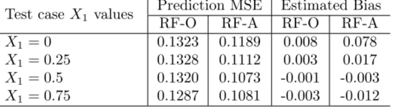
and actual test responses. Averaging these (average) prediction errors and biases produced the MSEs and estimated biases listed in Table 1. As Table 1 shows, augmenting with an irrelevant explanatory variable
X2 ∼U(0,1) reduced the prediction MSE at each of the four test sampleX1 values. The improvement
was more obvious for the predictions with anX1value in the middle of this variable’s range[0,1], rather
than at the edges.
Table 1: Predictions by the RFs grown from the original (RF-O) and augmented (RF-A) datasets.
Test caseX1 values
Prediction MSE Estimated Bias
RF-O RF-A RF-O RF-A
X1= 0 0.1323 0.1189 0.008 0.078
X1= 0.25 0.1328 0.1112 0.003 0.017
X1= 0.5 0.1320 0.1073 -0.001 -0.003
X1= 0.75 0.1287 0.1081 -0.003 -0.012
To begin to understand the results in Table 1, we recall that, as mentioned in Section 1 for the regression case, a prediction by a RF amounts to an average of the predictions produced by the trees in the forest, where each tree is grown from an independent bootstrap resample of the original data. Because
each tree prediction corresponds to some average of the responsesY1, . . . , Yn observed in the original
training data (i.e., the average of responses in a node from the dataset used to grow the tree), we can view
the final prediction of the RF (at some given level of explanatory variablesx0) as a convex combination
of the training responses
ˆ Y(x0) = n X i=1 wi(x0)Yi (8)
involving nonnegative weights wi ≡ wi(x0) with P
n
i=1wi = 1. The weights wi are functions of the
training sample and the regressor value of the test case x0. A single tree in the forest is grown by
a series of partitions of the regressor space (i.e., binary splits), which tend to pool data cases with similar regressors in the same nodes. As a result, a RF predicts a new case by selecting training cases over each tree that are close in terms of the explanatory variables, essentially producing a weighting
schemew1, . . . , wn that attempts to put more weight on responsesY1, . . . , Yn in the training dataset with
explanatory variables that match those at which a prediction is desired. RFs created with or without augmentation predictor variables (i.e., RF-A or -O) are attempting to produce weights that achieve a good
prediction of the responseY0≡Y0(x0)at some given level of the regressors. Lettingw= (w1, . . . , wn)T
andY = (Y1, . . . , Yn)T, the quality of a predictor Yˆ ≡Yˆ(x0)=P n
responseY0in terms of MSE, given by
E(Y0−Yˆ)2 = V ar(Y0) +V ar( ˆY) + [E( ˆY)−E(Y0)]2
= V ar(Y0) +V ar(wTY) + [E(wTY)−E(Y0)]2, (9)
depends on the weightswthrough the varianceVar(Yˆ) and biasE( ˆY)−E(Y0)of the predictorYˆ =wTY.
As in other regression problems, a trade-off exists in the RF method between prediction bias and variance, which are induced in this case by the selection of weights.
For the same simulation study that produced the prediction MSEs in Table 1, we can closely examine the weights (8) assigned to the training cases in a RF construction. Recall that each of the 101 training
observations in this study corresponds to a unique value of a non-random explanatory variable X1 =
i/100, i= 0, . . . ,100, chosen to equally partition the interval [0, 1]. Hence, from 1000 simulation runs,
we determined the average value of a weight wi assigned by a RF to a response Yi corresponding to
explanatory variableX1 =i/100, i= 0, . . . ,100, when trying to predict a new responseY generated at
each of theX1levels 0, 0.25, 0.5, and 0.75 listed in Table 1. The results are displayed in Figure 1 for both
RF-O and RF-A. Again, this figure gives an idea of how RFs with or without augmentation variables tend to select and weight training cases that are close in the regressor space to the positions at which
predictions are desired. Also included in Figure 1 for comparison are the optimal weightsw0, . . . , w100≥0
withP100
i=0wi= 1which minimize the prediction MSE (9); these values were computed numerically based
on knowledge of the true mean responseE(Y|X1)and varianceσ2, so such weights could not be used in
practice. However, optimal weights are useful for comparison against RF weighting schemes.
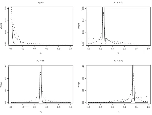
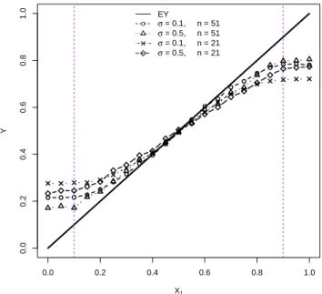
Figure 1 illustrates the reason for the improvement to RF by independent predictor variable augmen-tation. When predicting a test case, RF-O tended to concentrate weights only on a few training cases
withX1values immediately neighboring theX1value of the test case; in contrast, RF-A tended to spread
nonzero weights on more training cases. This often led to slightly more bias but substantially less variance
for RF-A predictions. For predictions of a new response at X1=0, RF-A clearly led to more bias (see
Table 1) because the weights on training cases could be only spread to training cases with a mean response
greater than the mean response atX1=0. But, in this study, bias cost much less than the gains made in
increased precision, and hence a uniformly smaller MSE was obtained by RF-A. In Figure 1, the inclusion
ofX2dragged the weight assignment in RF-A from the narrow assignment of RF-O towards the optimal
one. This weight-spreading effect helped to incorporate more training cases that were appropriately close
Figure 2: Average weights on responses in the training set (identified by theirX1 values) that contribute
to a prediction by either RF-O (–) or RF-A (- -). The dotted line (· · ·) corresponds to the weights used
by the best linear predictor of the form (8) that minimizes prediction mean squared error given in (9).
0.0 0.2 0.4 0.6 0.8 1.0 0.00 0.05 0.10 0.15 X1 = 0 X1 Weight 0.0 0.2 0.4 0.6 0.8 1.0 0.00 0.05 0.10 0.15 X1 = 0.25 X1 Weight 0.0 0.2 0.4 0.6 0.8 1.0 0.00 0.05 0.10 0.15 X1 = 0.5 X1 Weight 0.0 0.2 0.4 0.6 0.8 1.0 0.00 0.05 0.10 0.15 X1 = 0.75 X1 Weight
We also tried augmenting the dataset with different numbers of independentU(0,1)predictors. When
the number of irrelevant predictor variables was not very large (2 to 5), the prediction MSE for RF-A
was smaller than for RF-O for test cases with X1 values away from the 0 or 1 edges of this variable’s
range, but the degree of improvement was less than that shown in Table 1. This further augmentation had a less substantial effect in reducing the variance of predictions, as balanced against the corresponding losses in predictor accuracy. Furthermore, as the number of irrelevant predictors further increased (e.g., larger than five), the weights on responses in the training sample used for prediction became increasingly uniform. In these cases, bias increased and overwhelmed potential reductions in variance, leading to poor
prediction performance except for predictions atX1 values near the center of the [0, 1] interval, where a
uniform weighting is optimal (results not shown).
To further describe how augmenting the design matrix affects weight-spreading in RF predictions, it is helpful to provide some details on how trees in the forest are grown. The description provided here
is consistent with the default settings of the R packagerandomForest (Liaw and Wiener 2002). In the
RF procedure, a bootstrap resample of the training sample is used to grow a tree by a series of node splits, where to determine a node split, the algorithm considers a series of binary partitions composed from a set of randomly chosen predictor variables and their values. Consistent with Breiman (2001a), the
number of randomly selected predictors considered for each split is max{1,bp/3c} for regression, where
pis the total number of predictors. A node split is selected from the midpoints of the intervals between
ordered values from the randomly selected predictors (from a set of available cases), and two nodes are subsequently defined by splitting the values from the predictor variable into two disjoint intervals along a selected midpoint.
As an example, suppose a node is to be split, consisting of three training cases with two explanatory
variables: C1(X1 = 0, X2 = 0), C2(X1 = 1, X2 = 1), and C3(X1 = 2, X2 = 2). If we randomly
select the X1 variable for the split, then we would have two possible partitions, (−∞,0.5]∪(0.5,∞)
or (−∞,1.5]∪(1.5,∞), depending on the midpoint selected for the split. The mean surface for each
node/partition is estimated by the average response values over training cases in the node. The tree growing procedure is a greedy one, in that it always chooses the current best partition (midpoint for the split) in each step in order to minimize some loss criterion (i.e., squared error loss in regression), though this immediate best partition may not be the globally best one.
Consider the simulation of the last section, with two predictor variables (X2being the augmentation
variable). When growing both RF-O and RF-A, only one predictor (either X1 or X2) is randomly
selected for consideration at each split. Because the trees in RF-O construction must split only on the
right predictorX1, anarrow weighting scheme is induced, and the training cases ultimately weighted to
predict a new test case are very close to each other in terms of the distance between their X1 values.
On the other hand, with RF-A construction, bothX1 and X2 have equal chances to be considered at
a split. Splits based on the noninformative X2 variable may often direct the test case to a node that
does not contain the training cases closest to the test case in terms of distance between theirX1values.
Subsequent splits based onX1will tend to place the test case with training cases with similarX1values,
among those training cases that have not already been split onto different branches of the tree. In this
way, splits on the noninformativeX2 variable tend to diversify the tree structures and spread weights on
more training cases in prediction, which are roughly close to a new test case in terms ofX1 values (even
though splits on the variableX2 are not necessarily meaningful).
As an extremely simple illustration, suppose there are two training cases,C1≡C1(Y1, X1= 0, X2=
x21) and C2 ≡ C2(Y2, X1 = 1, X2 = x22) available for predicting an independent test case (Y3, X1 =
0, X2 = x23), where x21, x22, and x23 are realizations of iid U(0,1) random variables, and Y|X1 ∼
N(X1, σ2), similar to our previous simulation example. Consider three different possibilities for predicting
the test case response.
(a) A tree is grown on the right variableX1, with neither bagging nor predictor augmentation, which
prediction variance is2σ2.
(b) The RF-O prediction (i.e., using only X1) as a bootstrap expectation, based on bagging trees
grown from the following resamples {C1, C1}, {C2, C2} and {C1, C2} (with probability 1/4, 1/4, and
1/2), is3Y1/4 +Y2/4with prediction MSE given by4/64 + 104σ2/64, where the first and second terms in
the sum correspond to squared prediction bias and prediction variance, respectively. Note also here that the RF prediction, as a bootstrap expectation, was computed directly, without numerical approximation involving resampled trees.
(c) The RF-A prediction as a bootstrap expectation, based on bagging the same resampled trees as
RF-O but withX2augmentation, is given byY1/4 +Y2/4 +M/2, whereY1, Y2 andM are the outputted
predictions from resamples{C1, C1},{C2, C2}and {C1, C2}, respectively, withM defined as
M = 1 2Y1+ 1 2 Y1 ifx23≤(x21+x22)/2 andx21≤x22 Y2 ifx23≤(x21+x22)/2 andx21> x22 Y1 ifx23>(x21+x22)/2 andx21> x22 Y2 ifx23>(x21+x22)/2 andx21≤x22.
The dichotomous definition ofM owes to the fact that resample{C1, C2}offers two responses as potential
tree output and a tree is built from one regressor variable, randomly chosen betweenX1 and X2. For
this example, with respect to the iidU(0,1) draws defining the X2 variable, we would expect M to be
3Y1/4 +Y2/4 (interestingly matching the RF-O prediction in (b)), and we would then expect the final
RF-A prediction to be5Y1/8+3Y2/8, with MSE given by9/64+98σ2/64(again a two part sum consisting
of squared biases and prediction variance).
We see that the RF procedure itself (RF-O) assigns more weight onY2, when compared to a single tree
(no bagging), because bagging leads to unavailability ofC1 in some resamples. Augmenting the design
matrix with an independentU(0,1) variableX2 further spreads the weights fromY1 toY2, because the
possibility of splitting onX2 increases the potential for Y2 to be used for prediction even whenC1 is in
the bootstrap resample. This example intuitively explains how predictor augmentation helps to spread
weights on training samples in prediction. As the noise level σ2 increases, the RF-O method becomes
preferred (with respect to MSE) over a single tree, and RF with augmentation becomes preferred over
RF-O. More specifically, in this simple example, (a) has lowest MSE forσ2<1/6, (b) has lowest MSE for
σ2∈(1/6,5/6), and (c) has lowest MSE forσ2>5/6. Note that we do compromise prediction accuracy
(larger squared prediction bias) by implementing RF and additionally by predictor augmentation, but
issue in Subsection 4.2.
From the above argument, we also see that the weighting scheme of training samples used for pre-diction crucially influences the prepre-diction MSE, and this perspective also largely explains the prepre-diction improvements made by RFs over single trees in the first place. When the maximal node size is one, a tree typically predicts a test case using only one training case, and corresponds to the narrowest possible weighting scheme of the training responses. Bagging then helps to broaden the spread of weights in a convex combination of training responses as a predictor (8) based on training responses as long as the
number ofstructurally different trees is not too small. In a sense, this diversification of weights provides
a different, though related, perspective for understanding Breiman’s (2001a) original argument that RFs improve prediction by combining trees that are made less “correlated” (in Breiman’s words), or more diverse, by randomly selecting subsets of predictors (instead of using them all) to build trees. From a per-spective of weight-spreading, similarly structured trees, even if built by resampling, will tend to narrowly focus weights on a few training responses, while the prediction by more structurally diversified trees (i.e., diversified by randomly choosing regressor variables in resampled trees and, in our case, further diversi-fied by predictor variable augmentation) tend to positively weight a wider range of appropriate training cases and thereby reduce prediction variance. This again intuitively explains how RFs alleviate overfitting compared to an individual tree.
In the standard Monte Carlo (MC)-based implementation of a RF, where we numerically determine the RF prediction from a group of trees grown by a finite set of bootstrap resamples, we also note that there is a separate issue of using a sufficient number of trees (i.e., bootstrap resamples) to obtain a reasonable MC approximation, and the number of tree resamples can also impact the final weights used in a RF prediction in practice. However, simply increasing the number of resamples (or trees in a MC-constructed forest) only improves the MC-approximation to the weights assigned by a given RF procedure, and this does not change the structure of a RF-procedure itself (whether RF-O or RF-A). Our simulation study showed that the advantage of RF-A over RF-O in terms of prediction MSE remained unchanged when the number of resamples (trees per forest) increased from 100 to 10000 (results not shown). We will further discuss this issue of resample sizes in Sections 3 and 4.
3
Improvement by Variable Augmentation in Real Data
Exam-ples
While the previous section considered simulated data, improving test sample prediction performance of a RF by augmenting the design matrix with independent explanatory variables also occurs in real data analyses. For illustration, we first present some results based on the concrete compressive strength data of Yeh (1998). The dataset has 1030 observations, with eight quantitative input variables and a response variable, concrete compressive strength. We performed regression analyses (predictions) by RFs based on the original and augmented datasets, and we also examined the effect of maximal node size in the trees. We created 1000 independent partitions of the original data, where each time we randomly divided the data into a training set (with 1000 observations) and a test set (the remaining 30 observations) and
augmented the original design matrix with an independent U(0,1) predictor variable as in Section 2.
RF-A and RF-O were both grown with the maximal node size 1, 5, and 10 using the same 1000 training cases. The performance was evaluated based on prediction MSE of the test samples, averaging over test samples across the 1000 generated partitions. The results in Table 2 indicate that predictor augmentation reduced the prediction MSE, regardless of node size and number of trees in a RF. In this example, growing each tree to its largest possible form (maximal node size 1) produced better predictions than the default
setting (maximal node size 5) in the R packagerandomForest.
Table 2: Prediction MSEs in the concrete compressive strength regression with (RF-A) and without (RF-O) predictor augmentation.
Maximal node size
Prediction MSE RF-O RF-A 1 5 10 1 5 10 10 trees/resamples used 35.87 37.88 42.48 34.78 36.16 39.02 100 trees/resamples used 28.50 30.97 35.74 27.81 29.34 32.96 1000 trees/resamples used 28.42 30.98 35.73 27.67 29.29 32.94
Breiman (2001a) claimed that RFs do not overfit by showing its generalization error for a classification problem converges for an infinite number of trees. This suggests that increasing the number of trees in a RF is enough to solve the overfitting problem in RFs. Lin and Jeon (2006) showed that controlling node size improved prediction performance by RFs in some datasets. Table 2 shows that the relative performance of RF-O could not be improved either by increasing the number of trees per forest (resamples in the implementation of a RF), or increasing node size. The effect of node size and number of trees per RF will be further discussed in Subsection 4.1
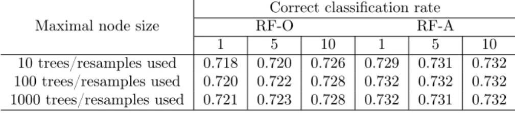
We also tested predictor augmentation in a classification problem with a real data set. Haberman (1976) reported a dataset on the survival of patients who had undergone breast cancer surgery at the University of Chicago’s Billings Hospital between 1958 and 1970. The dataset has three explanatory variables: age of patient at time of operation, year of operation, and number of positive axillary nodes detected. The binary response variable is patient’s survival status five years after operation. There are
306 patients in this dataset. Again we augmented the original design matrix with an independentU(0,1)
random variable. The dataset was randomly partitioned into a training set with 2/3 of the patients and a test set with the remaining 1/3 of the patients. We grew both RF-O and RF-A with the same training set and predicted the response in the test set with the maximal node size 1, 5, and 10. This process was repeated 1000 times, and the average correct classification rates are shown in Table 3. Augmenting the
design matrix with an independent U(0,1) predictor improved classification in all scenarios. As in the
previous regression problem with the concrete dataset, increasing the number of trees per forest led to
little or no improvement. The default maximal node size of therandomForest package for classification
problem is 1, which produced slightly worse predictions than the larger maximal node size considered for this dataset.
Table 3: Classification rates for Haberman’s survival data with (RF-A) and without (RF-O) data aug-mentation.
Maximal node size
Correct classification rate
RF-O RF-A
1 5 10 1 5 10
10 trees/resamples used 0.718 0.720 0.726 0.729 0.731 0.732
100 trees/resamples used 0.720 0.722 0.728 0.732 0.732 0.732
1000 trees/resamples used 0.721 0.723 0.728 0.732 0.731 0.732
4
Other Considerations Impacting the Effect of Variable
Aug-mentation
In Subsections 4.1 through 4.3, we briefly connect the evidence of improved random forest (RF) predictions by predictor augmentation to several other aspects influencing the performance of RFs, such as the number and size of individual trees in a forest, signal-to-noise issues, the dimensionality of data, and the functional relationship between mean response and explanatory variables. We also return to the issue of interpreting variable importance in light of variable augmentation in Section .
4.1
Number and size of trees
As described in Section 2, a RF grows an ensemble of trees with bootstrap samples and thereby improves prediction (over a single, less stable tree, cf. Breiman et al., 1989) by averaging a series of tree structures, and inducing a broader set of weights on training responses. We have seen that predictor augmentation can further add to tree diversification and weight-spreading in a RF predictor (8) and that, when such augmentation is helpful, it is because this acts to reduce prediction variance and mitigate overfitting. However, the issue of overfitting by RF has been debated since the method’s introduction. Breiman (2001a) claimed that RFs “never overfit” because RF generalization error for a classification problem converges as the number of trees increases. In our interpretation, this statement conveys that, as the number of resamples (and subsequent trees) increase in an MC-based implementation of RF, the numerical computation provides an increasingly better finite-sample approximation of the RF prediction, technically defined as a bootstrap expectation (cf. Section 1). This does not imply that RFs are immune to overfitting problems. Hastie et al. (2009) have shown that RFs can overfit despite increased tree numbers in an MC-implementation. Our predictor variable augmentation addresses a different issue than the number of trees in the RF construction, and we have illustrated that augmentation can improve predictions regardless of the number of trees.
Regarding tree size, Hastie et al. (2009) have also suggested that the overfitting of RFs with fully grown trees (i.e., maximal node size of 1) seldom costs much, especially in classification problems. It is commonly believed that RFs work best with a maximal node size of 1. However, the default maximal node
size values in the R packagerandomForest are 5 for regression and 1 for classification problems. Segal
(2004) and Lin and Jeon (2006) demonstrated minor gains in RF regression problems by controlling the node sizes of individual trees in a forest. In particular, Lin and Jeon (2006) related RFs to the adaptive k-nearest neighbor (kNN) method, and showed that tuning the maximal node size is advantageous for the performance of RFs. There can be an advantage of choosing a maximal node size larger than one for datasets with many observations but relatively small dimension, because this also has the effect of weight-spreading to reduce the variance of RF predictions. However, tuning the maximal node size of individual trees may not be enough to avoid overfitting problems in RFs completely, and predictor augmentation can still be beneficial with maximal node sizes larger than one. Our real data analysis examples in Section
3 (Table 2 and 3) indicate that prediction performance can be further improved by U(0,1) predictor
augmentation at different maximal node sizes. This suggests that, when such predictor augmentation is helpful, there may yet be room for improvement in RFs, including the choice of maximal node size.
4.2
Signal-to-noise issues and mean response function
The prediction variance for a given test case is, of course, related to the variance of the training data. More variability in the training data often translates into larger variances for RF predictions relative to their squared biases, and hence a larger benefit by predictor augmentation and widening the weights (8) on the training sample. In the simulation experiment of Table 1, for example, if we generate the response
variableY|X1 from N(X1,0.52) instead of N(X1,0.32), the variance/MSE reducing effect is even more
obvious by augmenting with an independentX2 from U(0,1). In contrast, ifY|X1 is fromN(X1,0.12),
there is hardly any improvement. That is to say, data sets with large signal to noise ratios benefit less from predictor augmentation.
Our simulation example in Section 2 was admittedly and intentionally simple in that the mean function
of response variable was linear in the only key predictorX1 equally partitioning the unit interval [0,1].
When the test sample has regressor values that are not too extreme so that there are training cases which approximately neighbor the test case in regressor space, averaging or weighting more training responses, induced by independent predictor augmentation, leads to better prediction precision without sacrificing too much prediction accuracy. However situations can arise where augmentation can hurt the overall prediction MSE because the gains in reduced prediction variance from weight-spreading cannot offset the damage in bias. This can occur, for instance, when the mean function is highly non-linear over small neighborhoods in the regressor space and the underlying noise is low. Consider another simple simulation
study, similar to that