Unsupervised learning for long-term autonomy

(1)

Copyright and use of this thesis

This thesis must be used in accordance with the provisions of the Copyright Act 1968.

Reproduction of material protected by copyright may be an infringement of copyright and

copyright owners may be entitled to take legal action against persons who infringe their copyright.

Section 51 (2) of the Copyright Act permits an authorized officer of a university library or archives to provide a copy (by communication or otherwise) of an unpublished thesis kept in the library or archives, to a person who satisfies the authorized officer that he or she requires the reproduction for the purposes of research or study.

The Copyright Act grants the creator of a work a number of moral rights, specifically the right of attribution, the right against false attribution and the right of integrity.

You may infringe the author’s moral rights if you: - fail to acknowledge the author of this thesis if

you quote sections from the work - attribute this thesis to another author - subject this thesis to derogatory treatment

which may prejudice the author’s reputation For further information contact the University’s Director of Copyright Services

(2)

Unsupervised Learning for

Long-Term Autonomy

Lionel Ott

A thesis submitted in fulfillment of the requirements for the degree of

Doctor of Philosophy

Faculty of Engineering and Information Technologies University of Sydney

(3)

Declaration

I hereby declare that this submission is my own work and that, to the best of my knowledge and belief, it contains no material previously published or written by another person nor material which to a substantial extent has been accepted for the award of any other degree or diploma of the University or other institute of higher learning, except where due acknowledgement has been made in the text.

Lionel Ott

(4)

Abstract

This thesis investigates methods to enable a robot to build and maintain an environment model in an automatic manner. Such capabilities are especially important in long-term autonomy, where robots operate for extended periods of time without human intervention. In such scenarios we can no longer assume that the environment and the models will remain static. Rather changes are expected and the robot needs to adapt to the new, unseen, circumstances automatically.

The approach described in this thesis is based on clustering the robot’s sensing information. This provides a compact representation of the data which can be updated as more information becomes available. The work builds on affinity propagation (Frey and Dueck, 2007), a recent clustering method which obtains high quality clusters while only requiring similarities between pairs of points, and importantly, selecting the number of clusters automatically. This is essential for real autonomy as we typically do not know “a priori” how many clusters best

represent the data.

The contributions of this thesis are three fold. First, a self-supervised method is presented that automatically builds a visual appearance model of the envi-ronment with traversability information of objects within the envienvi-ronment. The model allows the detection of obstacles in new observations for safe navigation. Improvements over existing large scale affinity propagation extensions are made with meta-point affinity propagation, reducing computational time and improv-ing robustness to noise. Experiments on indoor and outdoor data demonstrate the quality of the model as well as the ability to recognise obstacles. The useful-ness in long-term autonomy is demonstrated on outdoor data captured months apart.

Second, an extension of affinity propagation capable of clustering multiple data sources automatically is described. The method only requires information on a per sensor basis, which is automatically combined into a single clustering solution. This is of particular interest in robotics, as robots generally obtain data from different sensors. Experiments on indoor and outdoor RGB-D data demonstrate the advantage of combining multiple sensor modalities and the quality obtained by the proposed method in tasks such as segmentation and clustering.

Third, joint clustering and anomaly detection is formulated as a generic inte-ger program to which two optimisation methods are proposed. The formulation

(5)

automatically selects the number of clusters as well as a user defined number of meaningful outliers while only requiring pairwise similarities as input. The first solution is formulated using the affinity propagation framework while the second uses the Lagrangian duality which provides guarantees on the optimality of the solution. The benefits and properties of the proposed methods, including opti-mality, scalability and robustness, are shown on synthetic data. Applicability to real data is demonstrated on various real datasets such as hurricane GPS traces, MNIST digits, and New College image dataset.

(6)

Acknowledgements

First and foremost I would like to thank my supervisor Fabio Ramos for the opportunity to pursue a PhD with him, as well as his readily available support during the four years. The ability to explore freely while always having the ability to get feedback was immensely helpful.

I would also thank the University of Sydney and NICTA for the scholarship which allowed me to undertake this research.

I would also like to thank all the other students in Fabio’s group for interesting chats on various topics and especially the trips to the Field Lab for a dose of coffee. Thanks also to my family, which offered support despite being at the other side of the globe.

(7)

Nomenclature

Notation

The following is a listing of the notation used throughout this thesis. General X matrix x vector xT transpose of vector_x kxk L2 norm of vector _x |x| cardinality ofx

N number of points in a dataset

` number of outliers

k number of clusters to select

µ centroid of a cluster

N(µ,Σ) normal distribution with mean µand covariance Σ

Bk _k-th laser scan bin

Bk

i i-th measurement of thek-th laser scan bin

S laser scan Spectral clustering S similarity matrix G similarity graph D degree matrix W weight matrix

L graph Laplacian matrix

(8)

Convex optimisation

f, g, q functions

x function input

x[t] function input at time _t

X value range of x

L Lagrangian function

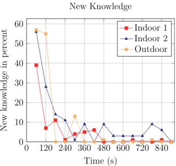
λ Lagrangian multiplier

f∗, q∗ optimal function values u[t] step size at time_t

∆x[t] step direction at_x at time _t

∇f(x) gradient off atx s[t] subgradient at time_t

δf(x) subdifferential off atx

Features and metrics

d(i, j) distance between point iand j

l, a, b LAB colour space values

x, y image pixel coordinates

H histogram

H entropy

I image

p image pixel

(9)

Affinity propagation

C(e, a), C(X) cost of specific solution

e exemplar choices

a assignments of points to exemplars

X binary assignment matrix

xij assignment matrix value in row icolumn j

I, E, S, Q, P factor nodes

L layer in layered affinity propagation

βij, ηij, ρij, αij,

τij, ωij, χik, λik,

τik, ωik

factor graph message

S similarity matrix

sij similarity value between point i and j

µv→f variable to factor message

µf→v factor to variable message

f factor in a factor graph

v variable node in a factor graph

Mlong long term model represented by streaming affinity propagation

Mshort short term model represented by affinity propagation

θmin-points minimum number of points required for a meta-point to be

consid-ered during the clustering

θsimilarity radius of a meta-point sphere

P set of points used for clustering with MPAP N set of points considered noise with MPAP Lagrangian duality

cj cost of selecting point j as exemplar

dij cost of assigning point i to exemplar j

o outlier indicator vector

A constraint matrix

F LOLP optimal solution value of the linear program

F LOLR optimal solution value of the Lagrangian relaxation

(10)

Abbreviations

AP Affinity propagation

APOC Affinity propagation outlier clustering BIC Bayesian information criterion

FLO Facility location with outliers

GPS Global positioning system

IMU Inertial measurement unit

IP Integer program

LAP Layered affinity propagation

LBP Local binary pattern

LD Lagrangian duality

LDA Latent Dirichlet allocation

LOF Local outlier factor

LP Linear program

LR Lagrangian relaxation

MAP Maximum a posteriori

MPAP Meta-point affinity propagation

RANSAC RANdom SAmple Consensus

ROC Receiver operating characteristic STRAP Streaming affinity propagation

(11)

List of Figures

1.1 Contemporary robots . . . 2

1.2 Image exemplars . . . 3

1.3 Affinity propagation example . . . 4

2.1 Affinity propagation graphical model . . . 12

2.2 Affinity propagation example . . . 16

2.3 Visualisation of the convexity definition . . . 17

2.4 Image subdivision method examples . . . 22

2.5 Histogram examples . . . 26

3.1 Examples of image patches . . . 32

3.2 Processing pipeline overview . . . 36

3.3 Heuristic motion decision examples . . . 40

3.4 Adding points into the meta-point system . . . 42

3.5 Clustering method example comparison . . . 45

3.6 Cluster location visualisation . . . 47

3.7 New knowledge over time . . . 48

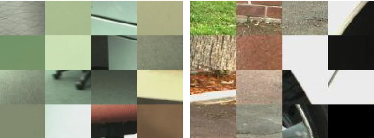
3.8 Exemplars identified in outdoor and indoor data . . . 49

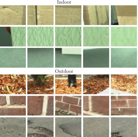
3.9 Cluster members in indoor and outdoor data . . . 50

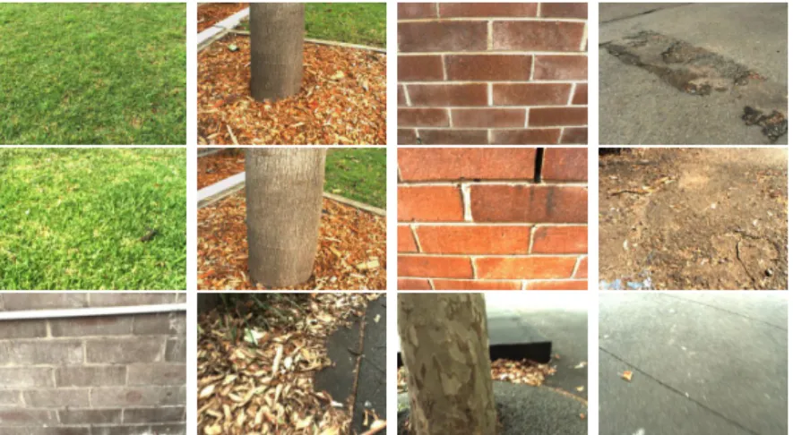
3.10 Images of experimental areas . . . 51

3.11 New knowledge when re-visiting areas . . . 52

3.12 New knowledge when re-visiting areas months later . . . 53

3.13 Laser collision avoidance processing pipeline . . . 54

3.14 Examples of laser scan and image data . . . 57

3.15 Collision prediction over time . . . 58

3.16 Laser feature evaluation for collision prediction . . . 58

4.1 Affinity propagation and layered affinity propagation messages . . 62

4.2 Factor graph of layered affinity propagation . . . 62

4.3 Kinect data segmentation results . . . 67

4.4 Clustering statistics visualisation . . . 69

4.5 KITTI point cloud examples . . . 71

4.6 Point clouds segments . . . 72

(15)

4.8 KITTI data clustering errors . . . 73

4.9 LAP and AP energy evolution . . . 74

5.1 Affinity propagation with outlier clustering graphical model . . . 81

5.2 Lagrange relaxation constraint matrix . . . 86

5.3 Clustering with outliers example . . . 90

5.4 Impact of data dimensionality on quality . . . 91

5.5 Impact of misspecified ` on quality . . . 92

5.6 Speed-up over LP, absolute runtime and per iteration runtime . . 92

5.7 Hurricane data clusters and outliers . . . 94

5.8 Evolution of λ for exemplars and outliers . . . 95

5.9 MNIST data clusters and outliers . . . 96

5.10 Clusters and outliers in the New College dataset . . . 98

5.11 Clusters and outliers in the New College dataset with Freiburg outliers . . . 99

(16)

List of Tables

2.1 Histogram distance values . . . 28

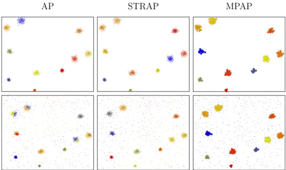
3.1 Clustering results of AP, STRAP, and MPAP . . . 46

3.2 Data ordering impact on clustering quality . . . 46

3.3 MPAP runtime breakdown . . . 51

3.4 Area under (ROC) curve . . . 55

4.1 Kinect data segmentation . . . 68

4.2 Features used on Kinect and KITTI data . . . 69

4.3 KITTI clustering results . . . 74

5.1 Advantages and disadvantages of clustering methods . . . 89

5.2 MNIST data results . . . 96

(17)

List of Algorithms

1 k-means . . . 9

2 Spectral clustering . . . 10

3 Affinity propagation . . . 15

4 Gradient descent . . . 19

5 Lagrangian dual function optimisation . . . 20

6 SLIC . . . 23

7 Earth Mover’s distance . . . 27

8 AP & STRAP integrating a novel observation . . . 39

9 MPAP add new observation . . . 44

10 Layered affinity propagation . . . 65

11 Affinity propagation with outlier selection . . . 82

(18)

Chapter 1

Introduction

Robotics has evolved drastically over time, from tools used to automate manufac-turing to autonomous rovers exploring Mars and self-driving cars. This would not have been possible without the advances and development of sophisticated hard-ware, from improved robotic designs to sensors such as IMU, cameras and laser scanners, associated with theoretical developments in machine learning. Chal-lenges to the robotics community, such as the ones organised by DARPA, play a significant role in advancing what is currently feasible. Projects such as the Google car would hardly be at the point they are today without those challenges. Robots are also becoming ubiquitous in every day life, from automated vacuum cleaners to small quadrotors. This means that robots are used in areas and ways that were not thought possible only a short time ago, naturally creating new chal-lenges, such as operating robots for extended periods of time with no or minimal supervision by humans. The availability of robots to non experts also highlights the importance of methods that do not rely on highly specialised knowledge to obtain good results. Robotics has always been a field which combined research from many different fields. Machine learning, supervised learning methods in particular, have been used extensively thanks to their ability to build accurate models from labelled data. However, for long-term autonomy, the big question is how can robots operate in unknown, changing environments without requiring human supervision?

1.1 Motivation

With robots being deployed to operate longer, with less human supervision, and by non-experts, methods with the ability to adapt become paramount. In such scenarios an important question is how models built based on training data can adapt to changes in the environment? One solution is to label more data and retrain the model. However, this is not appealing in the context of long-term autonomy due to the required human involvement. Unsupervised learning meth-ods, capable of automatically building and adapting a model, are an interesting solution to these problems. Such methods are not without challenges, as data

(19)

(a) Mars Rover (b) Google Car (c) Parrot AR Drone

Figure 1.1: Contemporary robots of varying complexity deployed in different sce-narios. From Mars rovers (a) (courtesy NASA/JPL-Caltech) to the autonomous Google car (b) (Courtesy of Wikimedia Commons) to recreational drones (c) (http://www.parrot.com/).

needs to be processed continuously and with limited control over the data being gathered. Clustering methods are good candidates as they typically make little to no assumptions about the data, and purely work on distance metrics to group the data into groups. This allows the clusters, or the model, to change as more and different data is observed.

The use of unsupervised methods has other advantages in addition to adapting to changes. There is no need for an initial model to exist and, as such, enables the creation of models entirely from scratch. This is particularly appealing for deployments in previously unvisited or inaccessible areas, such as other planets or disaster zones. Finally, such methods are suitable for use by non experts as they can independently learn a model after being deployed.

In another scenario, assume a robot equipped with a camera and a bump sensor is required to build a model that allows it to safely navigate the environment, i.e. without collisions. A typical supervised approach would label images collected in the environment with obstacle information, and train a classifier based on this data, allowing the robot to identify obstacles in images. However, as soon as the environment changes the model is no longer valid. Using unsupervised methods this issue can be avoided altogether. At the beginning, the model is empty and has to be built incrementally by observing the environment. Clustering images can be used to build a model of the environment, however, the information needed to classify parts of the environment as obstacles or non-obstacles is still missing. This information is added by incorporating the bump sensor in a self-supervised manner. Whenever the robot collides with the environment the bump sensor is triggered and the currently observed image data is labelled as belonging to ob-stacles. Over time the robot will accumulate this information in the clusters and be able to infer that certain clusters belong to obstacles. As time continues fewer collisions will occur, as the model will be able to classify observations correctly

(20)

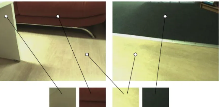
Figure 1.2: Example of the exemplars and their relation to parts of the image. into obstacles and non-obstacles. Figure 1.2 shows what such a model looks like, the small image patches indicate the clusters, corresponding to different objects in the environment. The two patches on the left represent obstacles while the two on the right correspond to non-obstacles. All of this happens without human supervision and is therefore amenable to adaptation in a changing environment.

1.2 Affinity propagation

Clustering algorithms, on which methods developed in this thesis are based on, group data points into clusters according to how similar or close they are to each other. Clustering methods typically require the user to provide the number of clusters to create beforehand, which is impossible for applications such as the one described above. Affinity propagation (Frey and Dueck, 2007) is a clustering method that does not require this information and works solely based on the distances between pairs of data points.

A short overview of affinity propagation is provided here with more details available in Section 2.2. Affinity propagation requires a square similarity matrix which contains the similarity or distance between all pairs of points as input and produces clusters and exemplars – the most representative point of a cluster – as outputs. Based on the similarity matrix a factor graph is built representing the clustering problem. The goal is to find the maximum a posteriori solution

to the factor graph which is achieved through message passing, which propagates messages between the nodes in the factor graph. The messages represent two intuitive measures: availability, sent from point k to point i, indicates how

ap-propriate it is for a point i to choose k as its exemplar, and responsibility, sent

from point ito point k, indicates how suitablek is as an exemplar for i. By

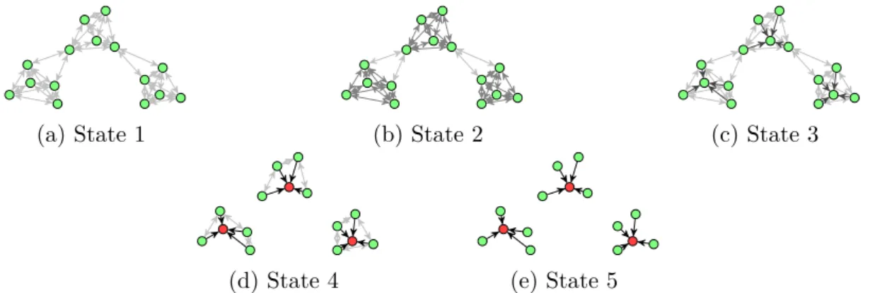
iter-atively updating these two messages across the entire graph a clustering solution emerges over time. The evolution of this process is depicted in Figure 1.3, where circles indicate the different data points, and arrows the availability messages,

(21)

(a) State 1 (b) State 2 (c) State 3

(d) State 4 (e) State 5

Figure 1.3: Different states in an exemplary run of affinity propagation. The ar-rows indicate the availability message sent from one point to another. Darker arrows indicate a higher message value. At the beginning no point is better suited to be an exemplar then any other, then over time, by passing messages, the most appropriate exemplars, marked in red, emerge.

with darker ones having higher belief value. Over time the clusters disconnect from each other and the exemplar points emerge.

While affinity propagation allows us to cluster data without providing an ex-plicit number of clusters, it has drawbacks over simpler clustering methods such as k-means. The biggest drawback is runtime, which is quadratic in the number

of data points making scaling to large amounts of data, and incorporating new data in a streaming manner, challenging. Additionally, the formulation of affin-ity propagation makes extensions challenging. Finally, affinaffin-ity propagation has to cluster all data points which can be problematic in the presence of noise.

1.3 Problem statement

In its most general form the problem addressed in this thesis is: how to enable a robot to learn and maintain a model of the environment autonomously. Building the model should not require any human supervision. The methods should be incremental and run in real-time. Not relying on human supervision allows the robot to be used in a much wider range of applications while incremental opera-tion allows the robot to adapt to changes without throwing away previous efforts. The very general nature of these requirements makes the developed methods us-able within a wide range of sensors and data, including cameras, laser scanners, GPS traces, and more. The models built in this way can be augmented with ex-periences made by the robot in a self-supervised manner, resulting in models that are automatically customised to the robot’s sensors and the task to be performed.

(22)

1.4 Contributions

This thesis addresses the challenges outlined above and makes contributions to clustering in general with applications to long-term autonomy. In the following we detail each of the contributions.

1.4.1 Self-supervised model learning

Robots operating for extended periods of time require methods that enable them to build and maintain a model of the environment without human supervision. We propose to address this problem using unsupervised methods, namely cluster-ing. As the methods need to operate without human input a clustering method capable of automatically selecting the right number of clusters is needed, affinity propagation in this case. Using this method an appearance model of the envi-ronment is built by clustering images observed by the robot. In order to provide information about whether an object is and obstacle or not the bump sensor on the robot is used in a self-supervised manner to annotate clusters with collision information. This allows building an appearance model with obstacle information without human supervision.

While affinity propagation produces good results it has quadratic runtime in the number of data points, which makes it impractical for real-time use in robotics. To address this problem an extension, meta-point affinity propagation, is intro-duced which reduces the amount of data points considered, and thus runtime, significantly. An additional benefit of this method is that it allows handling outliers, which affinity propagation is not capable of.

1.4.2 Multi-sensor clustering

Clustering algorithms typically require the user to provide distance information for pairs of points. In robotics, however, often times the goal is to cluster multiple data sources jointly which requires building and tuning a function that weights the different data sources against each other, before providing the clustering method with the combined distance values. This process is time consuming and does not generalise easily to different sensor configurations or datasets. The thesis addresses this with an extension to affinity propagation which requires only the distances between pairs of points for each sensor individually. Combing the dis-tances into a single clustering solution is performed by the clustering method in a way that obtains the best possible solution considering all the sources without any further tuning.

This makes processing multi modal data convenient and approachable. Experi-mental evaluation on RGB-D data shows the benefits of using multiple modalities

(23)

and the quality of the results obtained by selecting a clustering solution that is optimal with respect to all data modalities.

1.4.3 Joint clustering with outlier selection

A common phenomena in robotics data is noise, which often times is reduced by filtering the data. However, noise or outliers can also provide us with information. To address this an integer program formulation of clustering with outlier selection is presented. The goal of this is to cluster the data while removing a fixed number of points from the dataset which are the most likely outliers. In doing so the clustering problem becomes easier and more robust while at the same time information about the outliers in the data is preserved.

Two methods to solve the integer program are presented, one based on an extension of affinity propagation to outlier clustering, the other based on the Lagrangian relaxation of the integer program. The Lagrangian method exhibits additional appealing properties such as provable optimality, convergence guar-antees, and ease of parallel implementation. Experiments extensively test both methods on both synthetic and real datasets, demonstrating the ability to reveal interesting outliers as well as obtaining near optimal solutions at the fraction of the computational cost required by typical linear program solvers.

1.5 Outline

This chapter showcased how robotics is moving towards longer term deployments with less access to expert human supervision and therefore requires methods capable of unsupervised learning. Affinity propagation is a clustering method that provides a good base to build upon for these goals. This thesis takes advantage of the strengths of affinity propagation while improving its weaknesses and extending it for use in robotics applications.

Chapter 2 provides background knowledge necessary to the understanding of the thesis. Starting with clustering methods in Section 2.1 before describing affin-ity propagation and its extension to streaming, streaming affinaffin-ity propagation, in Section 2.2. Section 2.3 provides an overview of convex optimisation and subgra-dient optimisation. Image data pre-processing methods are detailed in Section 2.4 while Section 2.5 describes the different feature extraction and comparison meth-ods used in the thesis. Finally, Section 2.6 details the evaluation metrics used throughout the thesis.

Chapter 3 presents a system capable of learning a model of the environment and deciding if objects represent an obstacle to the robot without human super-vision. Additionally, meta-point affinity propagation is presented as an extension

(24)

to affinity propagation which significantly improves the computational perfor-mance. The problem is introduced in Section 3.1 and related work is discussed in Section 3.2. The system itself, using affinity propagation and streaming affinity propagation, is discussed in Section 3.3 before the meta-point affinity propaga-tion (MPAP) extension is discussed in Secpropaga-tion 3.4. Experiments in Secpropaga-tion 3.5 demonstrate the advantages of MPAP, as well as, the capability of the proposed system to learn and maintain a model based on data collected several months apart.

Chapter 4 generalises affinity propagation to allow multiple data sources to be clustered jointly without having to specify a joint cost function. Section 4.1 introduces the problem together with related work in Section 4.2. The graphical model and messages required for the method, layered affinity propagation, are derived in Section 4.3 based on the binary variable model (Givoni and Frey, 2009). Experiments in Section 4.4 demonstrate the capabilities of the method when segmenting and clustering RGB-D data.

In Chapter 5 a linear program formulation of the joint clustering and anomaly detection problem is introduced. The goal is to remove the most likely outliers in the dataset while automatically selecting the number of clusters. The prob-lem is introduced in Section 5.1 and related work is discussed in Section 5.2. Section 5.3 presents the integer program formulation alongside the derivation of the two methods of solving it: (i) a message propagation formulation and (ii) a Lagrangian duality based method. A proof of the optimality of the Lagrangian method as well as a comparison between the two methods follows. In Section 5.4 extensive evaluations on synthetic and real datasets demonstrate the behaviour of the methods and demonstrate the ability to reveal interesting outliers in the data while obtaining good clustering results.

The thesis concludes in Chapter 6 with a summary of the work presented in Section 6.1 and directions for future research in Section 6.2.

(25)

Chapter 2

Background

In this chapter we present the theoretical background of methods used throughout this thesis. In Section 2.1 we present clustering algorithms such as k-means and

spectral clustering. Section 2.2 gives an introduction to affinity propagation, the clustering method on which many of our contributions are built. This is followed by an overview of convex optimisation and its popular methods in Section 2.3. Section 2.4 introduces common image processing methods used to split an image into smaller patches, something commonly performed prior to feature extraction. Feature extraction and distance functions for use in clustering methods are ex-plained in Section 2.5. Finally, metrics used to compare clustering results are detailed in Section 2.6.

2.1 Clustering

Clustering is an unsupervised learning method that groups data according to the similarity of data points. As such clustering methods require the computation of the similarity or distance between pairs of data points. The number of clusters or groups found by the method are, based on the algorithm, either defined by the user or automatically determined at runtime.

2.1.1 k-means

k-means is a popular clustering algorithm consisting of the following two steps:

1. assign points to cluster centroids; 2. update centroids based on assignments.

These two steps are repeated until the assignments are stable. The algorithm requires the specification of the number of clusters. Algorithm 1 shows the steps performed by thek-means algorithm in more detail. First, thek initial centroids µi are selected (line 1 to 3). Next, points pi are assigned to the centroid closest

(26)

Algorithm 1: k-means

Input: data pointspi ∈P, number of clusters k,

number of data points N

Output: cluster centroids µ, cluster assignments a

1 for i_{∈ {}1, . . . , k_} do 2 µi ← pr ∈P 3 end 4 repeat 5 for i∈ {1, . . . , N} do 6 ai ← argminjkpi−µjk 7 end 8 for j _{∈ {}1, . . . , k_} do 9 µj ← (PipiI(i, j))/(PiI(i, j)) 10 end

11 until until convergence

12 return µ, a

This is repeated until a convergence criteria, such as no assignment changes, is fulfilled. The Ifunction in line 9 is an indicator function defined as follows:

I(i, j) =      1 if ai =j 0 otherwise. (2.1)

The result of the algorithm are k centroids with the points assigned to the

corre-sponding clusters.

The advantages of k-means are that it is a very simple and highly efficient

algorithm with a runtime of O(N), i.e. linear in the number of data points N.

Since the assignment of points to centroids is independent of each other this step can also be parallelised easily. The drawbacks of the method are its reliance on the user provided value fork as well as the need for good initial centroid selection.

A lot of work has been done in order to address these issues, such as using the Bayesian information criterion (BIC) to determine the number of clusters (Pelleg and Moore, 2000) or smart ways of selecting the initial centroids (Arthur and Vassilvitskii, 2007).

2.1.2 Spectral clustering

Spectral clustering refers to a group of algorithms operating on similar principles (see (von Luxburg, 2007) for a detailed overview). Here we describe a common version of the algorithm. Spectral clustering requires a similarity matrix which stores the pairwise similarities between pairs of points Sij = s(i, j). Based on

(27)

Algorithm 2: Spectral clustering

Input: similarity matrix S, number of clusters k

Output: clustering centroids µ, cluster assignments a

1 G_←BuildSimilarityGraph(S, condition) 2 for i, j _{∈ {}1, . . . , N_} do 3 if Gij = 1 then 4 Wij ←Sij 5 end 6 end 7 for i∈ {1, . . . , N} do 8 Dii ←PjWij 9 end 10 L←D−W 11 for i∈ {1, . . . , k} do 12 Ui ←EigenVector(L, i) 13 end 14 µ, a← k-means(U, k) 15 return µ, a

as-neighbourhood,k-nearest neighbours or full connectivity. The corresponding

weight matrix W is computed as Wij =Sij, ∀i, j :Gij = 1. Finally, the degree

matrix D of this graph is derived as follows:

Dii=

X

j

Wij. (2.2)

Based on the degree and weight matrices the graph LaplacianLis computed as:

L=D₋W. (2.3)

From the graph LaplacianL, we compute thek eigenvectors corresponding to the k smallest eigenvalues. These eigenvectors are then assembled into the new data

matrix U as follows:

U = [u1, . . . , uk]∈Rn×k, (2.4)

i.e. the eigenvectors make up the columns of U. Finally, this new data matrix U is clustered using k-means. Algorithm 2 shows the typical steps performed

during spectral clustering as pseudo code. The selection of the numberk, used to

select the number of eigenvectors and number of clusters is still topic of ongoing research. Common solutions such as, analysing the eigenvalues or eigenvectors has been shown to work well (Zelnik-Manor and Perona, 2004).

(28)

2.2 Affinity propagation

In this section we describe the affinity propagation method proposed by Frey and Dueck (2007) based on the binary variable model presented by Givoni et al. (2011). Affinity propagation is an exemplar based clustering method. This means that for each cluster a representative point, the exemplar, is selected. Addition-ally, affinity propagation also selects the number of clusters based on the pairwise similarities between points and the cost of cluster creation. The pairwise similar-ities and cluster creation cost are the only parameters the user needs to provide. We start by describing the approach from an optimisation point of view in Section 2.2.1. In Section 2.2.2, we described an algorithm for solving the problem using belief propagation (Pearl, 1988).

2.2.1 Optimisation view

Our goal is to find the set of exemplars e and assignments a of points to these

exemplars which maximises the cost C of the solution, i.e.:

C(e, a) = N X i=1 sim(i, ai) + k X j=1 cost(ej), (2.5)

where sim(i, ai) is the similarity between point i and the exemplar point ai,

cost(ej) is the cost of creating a cluster with point j as the exemplar, and k

is the number of clusters selected by the algorithm. Note that similarity and cost values need to be always negative, i.e. simij,costj <0. Points that are very

similar to each other have a similarity value close to 0. For this reason our goal is to maximise the cost function as this results in a solution which is as close to 0 as possible.

We can simplify Eq. (2.5) by representing the assignmentsa and exemplars e

by a binary assignment matrixX, wherexij = 1 indicates that pointiis assigned

to exemplar j and xjj = 1 denotes point j as an exemplar. Additionally we

combine the sim(i, j) and cost(j) functions into a single matrix as follows:

Sij =      cost(j) if i=j sim(i, j) otherwise. (2.6)

With these changes the cost function takes the form:

C(X) = N X i=1 N X j=1 Sijxij (2.7)

(29)

x

ij

S

ij

E

j

I

i sij αij ρij βij ηij (a) AP Messages E1 Ej EN x11 x1j x1N I1 Ii xN1 xN j xN N IN xi1 xij xiN S11 S1j S1N Si1 Sij SiN SN1 SN j SN N (b) AP Graphical Model

Figure 2.1: Visualisation of affinity propagation (a) messages and (b) complete factor graph. The factor graph shows how each row in the assignment matrix X is connected to a single I factor and similarly each column

is associated with a singleE factor node.

1. an exemplar must choose itself as its own exemplar; 2. points can only be assigned to valid exemplars;

3. every point can only be assigned to a single exemplar. This results in the following optimisation problem:

maximise XN i=1 N X j=1 Sijxij (2.8a) subject to X j xij = 1 ∀i (2.8b) xij ≤xjj ∀i, j (2.8c) xij ∈ {0,1} (2.8d)

In the next section we describe how Eq. (2.8) can be reformulated such that loopy belief propagation (Kschischang et al., 2001) can be used to solve it. 2.2.2 Graphical model view

Affinity propagation maximises the energy of Eq. (2.8) by representing the prob-lem as a factor graph, shown in Figure 2.1b. The nodes in the graph are the variable assignmentsxij while the factors encode the different constraints

enforc-ing a valid solution. The maximum a posteriori (MAP) solution is then computed using loopy belief propagation. The only input required is the similarity matrixS

which contains the similarity between pairs of data points and the cost of selecting a point as an exemplar on the diagonal.

The constraints imposed on a valid solution in Section 2.2.1 are formulated as follows:

(30)

1. 1-of-N Constraint (Ii). Each data point has to choose exactly one exemplar.

2. Exemplar Consistency Constraint (Ej). For point i to select point j as its

exemplar, point j must declare itself an exemplar.

Mathematically, these constraints are formulated as follows:

Sij(xij) =      Sij if xij = 1 0 otherwise (2.9) Ii(xi:) =      0 if P jxij = 1 −inf otherwise (2.10) Ej(x:j) =      0 if xjj = maxixij −inf otherwise (2.11) where xi:=xi1, . . . , xiN and x:j =x1j, . . . , xN j.

Combining these constraints with the user provided similarity values Sij, we

obtain the following energy function to be maximised: max X N X i=1 N X j=1 Sijxij + X i Ii(xi:) + X j Ej(x:j). (2.12)

In order to optimise this energy function with the max-sum algorithm we propa-gate messages through the factor graph. In their most general form, these mes-sages are defined as follows:

µv→f(xv) = X f∗_∈_ne₍_v₎_\_f µf∗_→_v(x_v), (2.13) µf→v(xv) = max_x 1,...,xM f(xv, x1, . . . , xM) + X v∗_∈_ne₍_f₎_\_v µv∗_→_f(x_v∗) , _(2.14)

wheref is a factor, or a function over a subset of variables,µv→f(x) is the message

sent from node v to factorf,µf→v(xv) is the message from factorf sent to node

v, ne() is the set of neighbours of the given factor or node, and xv is the value of

node v.

In Figure 2.1a it can be seen that each node xij is connected to three factors

Sij,Ii and Ej. The messages ρij and βij are sent from nodes to factors and thus

are derived using Eq. (2.13). The other three messages sij, αij and ηij are sent

from factor to node and need to be derived using Eq. (2.14).

In order to obtain an efficient algorithm we employ several strategies to sim-plify the computations needed to obtain the solution. Since we are using binary variables and absolute scale is not important it is sufficient to compute the

(31)

dif-ference between the two possible variable settings, i.e. αij = αij(1) −αij(0).

Furthermore, due to the construction of the two constraints in Equations (2.10) and (2.11) only certain assignments are possible which is exploited here to sim-plify the update equations. Combining these two ideas we arrive at the following update equations: sij =Sij (2.15) βij =sij +αij (2.16) ηij =−max k6=j βik (2.17) ρij =sij +ηij (2.18) αij =      P k6=jmax(0, ρkj) i=j minh 0, ρjj+Pk /∈{i,j}max(0, ρkj) i i6=j. (2.19)

This can be further simplified by expressing ρij as follows:

ρij =sij +ηij =sij −max

k6=j βik =sij −maxk6=j (sik+αik) (2.20)

Thus we have recovered the availability (α) and responsibility (ρ) messages of

the original affinity propagation formulation (Frey and Dueck, 2007). The two messages that need to be computed iteratively are therefore α and ρ.

The pseudo code for Algorithm 3 shows the steps performed by affinity prop-agation. The only input is the similarity matrix S which contains the point to

point distances on the off-diagonal as well as the cost of declaring a point an exemplar on the diagonal. The algorithm starts by initialising α and ρ messages

to 0 and then repeatedly updates ρ and α until convergence is achieved.

Con-vergence is typically achieved when the energy of the solution is stable over a number of iterations. Finding the MAP solution is performed by first extracting the exemplars and then assigning the remaining points to them. Exemplars are the points for whichαjj+ρjj >0, while the assignment of points to exemplars is

achieved by assigning pointito the exemplarewhich satisfies argmaxe(αie+ρie).

An example of the evolution of the belief represented by the algorithm about the MAP solution is shown in Figure 2.2. Circles represent the nodes while the darkness of the lines indicate the strength of the association of points to each other. Over time the links between nearby points strengthen identifying the exemplars, shown as red circles.

(32)

Algorithm 3: Affinity propagation Input: Similarity matrix S

Output: Exemplars e and assignmentsa

1 foreach i, j _{∈ {}1, . . . , N_} do 2 αij, ρij ←0 3 end 4 repeat 5 foreach i, j ∈ {1, . . . , N} do 6 ρij ←sij −maxk6=j(sik+αik) 7 end 8 foreach i, j ∈ {1, . . . , N} do 9 αij ←    P k6=jmax(0, ρkj) i=j minh 0, ρjj+Pk /∈{i,j}max(0, ρkj) i i6=j. 10 end 11 until convergence

12 e ← points for which (αjj+ρjj)>0 holds

13 ai ← assign point ito exemplar e satisfying argmaxe(αie+ρie)

14 return e, a

2.2.3 Streaming affinity propagation

While affinity propagation can compute solutions involving a few thousands data points in under a minute, it is not fast enough for use in real-time robotics applica-tions with a large number of observaapplica-tions. However, there are methods extending affinity propagation to handle data streams in real time, such as streaming affinity propagation by Zhang et al. (2008). The naïve approach to use affinity propaga-tion for data streaming would be to recompute the clustering with every newly observed data point. This obviously does not work when real-time performance is required. Streaming affinity propagation solves this problem with the following two ideas:

1. reduce the number of data points involved in the affinity propagation com-putation;

2. limit the number of times affinity propagation needs to be executed. These two goals are achieved by treating data points as one of two types, those that are similar to existing clusters and those that are dissimilar from the existing clusters. Points that are similar to an existing cluster are used to update the most similar cluster. Points that are dissimilar are added to an outlier reservoir which stores data points that currently cannot be represented by the clusters. Each cluster is described by a 4-tuple (ei, ni,Σi, ti) whereei is the exemplar associated

(33)

(a) State 1 (b) State 2 (c) State 3

(d) State 4 (e) State 5

Figure 2.2: Different states in an exemplary run of affinity propagation. The ar-rows indicate the availability message sent from one point to another. Darker arrows indicate a higher message value. At the beginning no point is better suited to be an exemplar then any other, then over time, by passing messages, the most appropriate exemplars, marked in red, emerge.

is the distortion of the cluster, and ti is the last time a point has been added

to the cluster. Once the outlier reservoir is full, affinity propagation is used to recompute the clustering. This requires the computation of similarity values between clusters and the points in the reservoir. These computations take the statistics stored in the clusters into account and are recomputed once affinity propagation has clustered the data. The net result of this approach is that the affinity propagation algorithm is executed less often and when performed, the number of data points involved is small.

2.3 Convex optimisation

Affinity propagation is an optimisation problem, which is solved using message passing, however, classic optimisation is another way to solve the problem. Con-vex optimisation in particular is appealing due to its properties and is used in Chapter 5 to perform clustering with outlier selection.

Convex optimisation (Boyd and Vandenberghe, 2009) is a field of optimisation concerned with the optimisation of convex functions. A function f :Rn 7→R is

convex if its domain is a convex set and if for all x, y _∈ domf with 0 _≤ θ _≤ 1

the following holds:

f(θx+ (1₋θ)y)_≤θf(x) + (1₋θ)f(y). (2.21)

A graphical interpretation of this expression is shown in Figure 2.3. Convex functions are desirable as they guarantee that a local optimum is also the global optimum, and as such, can be optimised using simple gradient based approaches.

(34)

f(x)

f(y)

θf(x) + (1₋θ)f(y)

x y

f(_·)

Figure 2.3: Visualisation of the convexity definition of Eq. (2.21). A general convex optimisation problem has the following form:

minimise f(x) (2.22a)

subject to gi(x)≤0, i= 1, . . . , m (2.22b)

x_∈X (2.22c)

where f is a convex cost function,gi the set of convex constraint functions and

X _⊂Rn a non-empty closed convex set.

2.3.1 Lagrangian relaxation

The formulation of Eq. (2.22) is called the primal problem. Introducing Lagrange multipliers λi ≥ 0 for the constraints gi, the Lagrangian can be written in the

following manner: L(x, λ) =f(x) + m X i=1 λigi(x). (2.23)

This forms a weighted sum of the objective and constraint functions with associ-ated Lagrange multipliers. The optimisation problem formed by the Lagrangian relaxation is called the dual problem and is of the form:

maximise q(λ) (2.24a)

subject to λ_≥0 (2.24b)

λ∈Rm, (2.24c)

where q(λ) is the dual function defined by: q(λ) = inf x∈X f(x) + m X i=1 λigi(x) . (2.25)

(35)

The optimal value of the primal problem is denotedf∗ while the optimal solution

to the dual problem is denoted as q∗. This formulation has the following useful

property.

Theorem 1. The dual function q(λ) is a lower bound to the primal solution for

λ_≥0, i.e.:

q(λ)_≤f(x∗) (2.26)

Proof. Consider a feasible solutionxe:

q(λ) = inf x∈XL(x, λ)≤ L(x, λe ) =f(xe) + m X i=1 λigi(xe) ≤f(xe) (2.27)

since gi(xe) ≤ 0 and λi > 0. Therefore, q(λ) ≤ L(x, λe ) ≤ f(xe) for all feasible xe and thus q(λ)_≤f(x∗) =_f∗.

From Theorem 1 we obtain q∗ _≤ _f∗. If the inequality is strict, i.e. _q∗ _{< f}∗

we have “weak duality”, which gives rise to the duality gap f∗ ₋_q∗. This gap

indicates how far apart the two solutions are. The second and more interesting case, where q∗ =_f∗, is called strong duality and implies that the solution of the

dual is equivalent to that of the primal. Strong duality is interesting, as it allows us to solve the primal problem to the optimality by solving another, potentially easier problem. In order for strong duality to hold the primal problem needs to satisfy the so called constraint qualifications.

All of the above becomes more useful when combined with the fact that the Lagrangian dual function q(λ) is always a concave optimisation problem, as its

objective function is the infimum of a family of affine functions inλ. This means

that we can apply standard gradient based optimisation methods to solve it. In the following we will introduce gradient descent and its adaptation to non differentiable functions, subgradient descent (Bertsekas, 1999).

2.3.2 Gradient descent method

One of the simplest methods for convex optimisation is the gradient descent method. Given a convex function f(x) the method generates a sequencex[t]_{, t}=

1, . . . with

x[t+1] =_x[t]+_u[t]∆_x[t]_, (2.28)

which minimises f. The update involves the “step size” u[t] _>0 and “step

(36)

Algorithm 4: Gradient descent

Input: function to optimise f, starting point x, stopping threshold η

Output: Optimal value of x

1 repeat

2 ∆x_{← −∇}f(x)

3 Select step size u >0

4 x _← x+u∆x

5 until _k∇f(x)_{k ≤}η

6 return x

∆x[t] =_−∇_f(_x). The “step size” can be found using a variety of methods such

as exact line search, backtracking line search, fixed step size or decreasing step size. Algorithm 4 shows the steps performed by gradient descent.

2.3.3 Subgradient method

As mentioned before the Lagrangian dual problem is a convex optimisation prob-lem, even if the primal problem is non convex. The optimisation problem though is piecewise linear and convex and therefore non differentiable, which is a require-ment for gradient descent based methods. However, we can sidestep this problem by using subgradient based methods.

The vectors is a subgradient of the convex function f :Rn7→R at x∗ if:

f(x)_≥f(x∗) +sT(_x

−x∗), (2.29)

for all x _∈ Rn. The subdifferential ∂f(x∗) is the set of all subgradients of f at x∗. Using subgradients we can optimise functions using gradient based methods

even if they are not differentiable. Algorithm 5 shows the general steps performed during subgradient optimisation of the Lagrangian dual function. The Lagrange multipliersλare initialised to random values before repeatedly (i) solving the dual

function, (ii) selecting one subgradient at the location obtained as the solution of (i) and then (iii) updating the Lagrange multipliers. This is repeated until the optimal solution is found, which is the case when the subdifferential contains the zero vector.

The method used to select the step size u[t] can have a significant impact on

convergence and optimality properties. When the step size fulfils the following

constraint: _∞ X t=1 u[t]=_∞ and lim t→∞u [t]= 0_, (2.30)

(37)

Algorithm 5: Lagrangian dual function optimisation Input: Optimisation problemq(λ)

Output: Optimal solution λ[t−1]

1 λ[0] _← random vector _∈ Rn+ 2 t _← 0 3 repeat 4 x∗ ← infx∈X{f(x) +Piλigi(x)} 5 Pick a subgradient s[t] at_L(_{λ, x}∗) 6 λ[t+1] _←max(_λ[t]₋_u[t]_s[t]_,0)_, _u[t]_>0 7 t ← t+ 1 8 until 0_∈∂q(λ[t]) 9 return λ[t−1]

size function that fulfils this constraint is the following,

u[t]=_u[0]_αt _α

∈(0,1). (2.31)

2.4 Image pre-processing

In this thesis we are often interested in modelling objects in scenes captured by images. As such it is desirable to break the image down into smaller patches to reduce the complexity contained in patch compared to the full image. There are many different approaches to this problem with different trade-offs in runtime and accuracy. In the following we present the two methods used in this work, equal subdivision and super pixel methods.

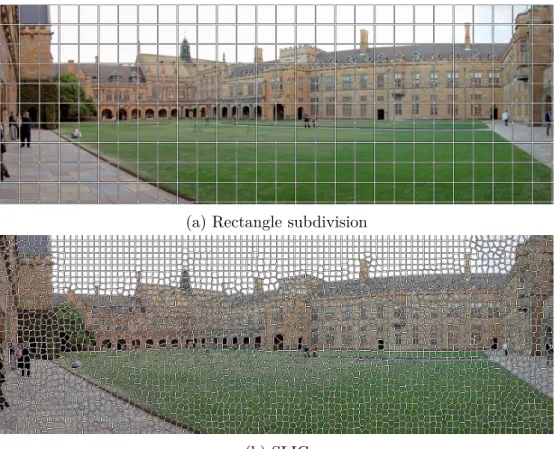
The visual difference of the patches these methods produce is shown in Fig-ure 2.4 where the top image is produced using equal subdivision and the bottom image with SLIC.

2.4.1 Equal subdivision

This is the simplest method to split an image into smaller patches. The original images is subdivided into a user defined number of equal sized rectangles covering the entire image. This method entirely ignores the contents of the image and, as such is inaccurate at finding borders of objects in a scene, however, it is extremely fast to compute.

2.4.2 Super pixel

Another popular approach is the use of super pixels. A super pixel is a collection of connected pixels in the image that are similar to each other. A super pixel

(38)

method segments the entire image into a collection of super pixels attempting to split the image along object borders. Commonly used methods include normalized cuts (Shi and Malik, 2000), watershed based methods (Vincent and Soille, 1991) and the recently proposed SLIC method (Achanta et al., 2012). In this work we use SLIC, as it has better runtime performance then alternative methods and produces good super pixels.

In the following we give a short overview of the SLIC algorithm. The basic idea of the algorithm is to run k-means on the image. Unfortunately, running

standard k-means would be too costly so a different strategy is adopted. The

assignment step of k-means is restricted in size around each centroid. The

algo-rithm requires two parameters, the number of super pixels k to be generated as

well as a compactness parameterm. The algorithm starts by seeding the initialk

centroids in a regular grid over the image. Next, the algorithm performs several rounds of k-means in a five dimensional space. The search space consists of the

three LAB colour channels of the image as well as the xand y pixel coordinates.

A special distance function is used, which normalises the colour and coordinate distance of pixels against each other, and has the following form:

dc(i, j) = q (lj −li)2+ (aj−ai)2 + (bj −bi)2 (2.32) ds(i, j) = q (xj −xi)2+ (yj−yi)2 (2.33) D(i, j) = v u u t dc Nc !2 + ds Ns !2 , (2.34)

where dc is the colour distance, ds the spatial distance, Nc the colour normaliser

and Ns the spatial normaliser. The spatial normaliser Ns can be defined as

the step size S, the initial distance between neighbouring centroids. The colour

normaliser Nc, however, is harder and is often left as a user defined compactness

parameter m. Using the normalisers NS =S and Nc =m the distance function

can be rewritten as:

D(i, j) = v u u td2 c + ds S !2 m2_. (2.35)

Tuning m allows to change the behaviour of the super pixels to either be more

compact, high value of m, or adhere more to image boundaries, low value of m.

(39)

(a) Rectangle subdivision

(b) SLIC

Figure 2.4: Examples of the two presented methods applied to an image of the University of Sydney’s Quadrangle. The white border indicates the individual patches.

2.5 Feature extraction and comparison

Typically raw sensor readings need to be processed before being used by other algorithms. This is done for several reasons. First, raw data can be too high dimensional to be used directly especially with images. Second, raw data may not be invariant to certain types of transformations, such as orientation or illu-mination which makes observations harder to relate to each other. Finally, raw data can be susceptible to noise which a pre-processing step can reduce.

2.5.1 Camera based features

Cameras are a very common passive sensor that provide colour and texture infor-mation about a scene and typically have high resolution and inforinfor-mation density. Extracting meaningful features from images is a topic of constant research and has evolved dramatically over the years. Examples include simple statistical fea-tures, such as the ones we will present here, finely tuned descriptors such as SIFT (Lowe, 1999), and recent advances based on deep belief networks (Lee et al., 2009) and convolutional neural networks (Krizhevsky et al., 2012).

(40)

Algorithm 6: SLIC Input: Step size S,

Output: Super pixel labels label

1 Initialise cluster centres µk ←[lk, al, bk, xk, yl] using step size S

2 foreach pixel i do

3 labeli ← −1

4 disti ← ∞

5 end

6 repeat

7 foreach Cluster centre µk do

8 foreach pixel i in a 2S_×2S region around µk do

9 if distance(i, µk)<disti then

10 disti ← distance(i, µk)

11 labeli ←k

12 end

13 end

14 end

15 Update cluster centres 16 until iteration limit reached

17 Fix connectivity and merge small super pixels 18 return label

extractor and the quality of the results obtained in a particular application. In the following we will describe very simple histogram based features, as they are very fast to compute and typically offer a reasonable description for our goals. Colour histograms

Colour histograms are a very simple way to concisely represent the intensity distribution of an image. The intensity value range is discretised into several bins of equal width and the value of each bin is based on the number of pixels that fall into it, i.e.:

Hi =

X

p∈I

δ(p), (2.36)

where Hi is the i-th bin,I the image and δ(p) the Dirac function that returns 1

if p is within the interval of Hi, and 0 otherwise.

Such a representation is good at capturing information on a global scope but loses all spatial information contained in the image. When considering colour images represented by multiple channels, such as RGB, HSV or LAB, different schemes can be used to represent them via histograms. One possibility is to create one histogram per channel and treat them separately. Another one is to build two or three dimensional histograms where each dimension represents a different channel. The choice of which representation is the best often depends on the size

(41)

of the image. This is due to the fact that in order to create a meaningful two or three dimensional histogram, a large number of data points, i.e. image pixels, need to be available.

Local binary patterns

As mentioned previously, colour histograms discard the spatial information con-tained in an image. As such the histograms for two images with identical amount of black and white but one organised as a chequerboard and the other one as two halves of solid colours would result in the same histogram. An attempt to rem-edy this problem are features which extract texture information from an image. Texture information is typically obtained by evaluating the gradients in a local neighbourhood of a pixel. Aggregating this gradient information into histograms allows us to capture the overall texture information of a single image.

Local binary patterns (Ojala et al., 2002) is a feature that builds such a texture representation. The feature is built by considering P neighbouring points which

are equally spaced on a circle of radius R around a central pixel. Based on this

the texture extractor is defined as:

T =t(gc, g0, . . . , gP−1), (2.37)

wheregcis the grey scale value of the centre pixel and g0, . . . , gP−1 are the values

of the neighbouring P pixels.

In order to obtain a feature invariant to global changes in grey scale values and rotation, the following steps are performed. First, the difference between the centre pixel and the neighbours is used, i.e.:

T =t(gc,(g0 −gc), . . . ,(gP−1−gc)). (2.38)

This is then simplified via the assumption that gi − gc is independent of gc,

yielding:

T =t(gc)t((g0−gc), . . . ,(gP−1−gc)). (2.39)

In practice this assumption is not warranted, however, it provides invariance to shifts in grey scale levels and allows us to remove gc from the texture extractor.

To further increase robustness only the sign ofgi−gc is considered resulting in:

(42)

where s(x) =      1 x_≥0 0 x <0. (2.41)

To encode the extracted texture with a single descriptor a binary representation is used, where the value 2i is assigned to each sign _s(_g

i−gc), i.e.: LBPP,R = P−1 X i=0 s(gi−gc)2i. (2.42)

This encoding results in 2P possible values. Rotational invariance is achieved

through a rotation scheme which aims to ensure that a maximal number of most significant bits, starting from gP−1, are 0.

In order to reduce the number of possible patterns and exclude those patterns occurring infrequently the concept of uniform patterns is introduced. The uni-formity of a pattern is based on the number of 0 → 1 transitions in the binary representation of a pattern. Only patterns with a uniformity score of 2 or less are used in the final representation, i.e.:

LBPU R,P =      PP−1 i=0 s(gi−gc) ifU(LBPP,R)≤2 P + 1 otherwise , (2.43)

where the uniformity score is computed as

U(LBPP,R) = |s(gP−1−gc)−s(g0−gc)|

+PX−1

i=1

|s(gi−gc)−s(gi−1−gc)|

. (2.44)

The result of this is that the P uniform patterns are mapped to bins 0 through P

while the remaining patterns are mapped to bin P + 1. The reason non-uniform

patterns are discarded is that they make up only a small portion of the observed patterns and it is therefore hard to obtain accurate statistics for them. To obtain the actual histogram representation of an image’s texture, the LBPU

P,R value is

computed for every pixel in the image. 2.5.2 3D laser point clouds

3D point cloud data is becoming more common, mainly due to the Kinect, an affordable structured light sensor. However, the Kinect is restricted to short ranges and indoor environments. In outdoor environments 3D point cloud data is therefore gathered by rotating planar laser scanners or Velodyne laser scanners.

(43)

0 1 2 3 4 0 10 20 30 40 (a) Histogram 1 0 1 2 3 4 0 10 20 30 40 (b) Histogram 2 0 1 2 3 4 0 10 20 30 40 (c) Histogram 3

Figure 2.5: Examples of histograms. Histograms (a) and (b) have similar shape but differ in absolute value while histogram (c) has entirely different shape and values. Using Euclidean distance this notion of shape of the distribution is not captured, however, using Bhattacharyya distance this information is considered in the computation.

Common to the data provided by all of these sensors is that they provide 3D points with no direct information about the structure they represent, which can make their interpretation challenging.

Surface normal histograms

Data collected in urban environments is full of planar surfaces, which can be characterised by their normals. As such a histogram over the surface normals can be a good feature in such situations. Before we can compute a surface normal histogram we need to compute the normal of each point in the point cloud. As mentioned before, point cloud data contains no information about the structure these normals are estimating. Several methods exist which use different assump-tions, an overview of common methods is given in Klasing et al. (2009).

Surface no