NetKet: A machine learning toolkit for many-body quantum systems

Contents lists available atScienceDirect

SoftwareX

journal homepage:www.elsevier.com/locate/softx

NetKet: A machine learning toolkit for many-body quantum systems

Giuseppe Carleo

a,∗

, Kenny Choo

b

_{, Damian Hofmann}

c

_{, James E.T. Smith}

d

_,

Tom Westerhout

e

, Fabien Alet

f

, Emily J. Davis

g

, Stavros Efthymiou

h

, Ivan Glasser

h

,

Sheng-Hsuan Lin

i

, Marta Mauri

a,j

, Guglielmo Mazzola

k

, Christian B. Mendl

l

,

Evert van Nieuwenburg

m

_{, Ossian O’Reilly}

n

_{, Hugo Théveniaut}

f

_{, Giacomo Torlai}

a

_,

Filippo Vicentini

o

, Alexander Wietek

a

a_{Center for Computational Quantum Physics, Flatiron Institute, 162 5th Avenue, NY 10010, New York, USA} b_{Department of Physics, University of Zurich, Winterthurerstrasse 190, 8057 Zürich, Switzerland}

c_{Max Planck Institute for the Structure and Dynamics of Matter, Luruper Chaussee 149, 22761 Hamburg, Germany} d_{Department of Chemistry, University of Colorado Boulder, Boulder, CO 80302, USA}

e_{Institute for Molecules and Materials, Radboud University, NL-6525 AJ Nijmegen, The Netherlands} f_{Laboratoire de Physique Théorique, IRSAMC, Université de Toulouse, CNRS, UPS, 31062 Toulouse, France} g_{Department of Physics, Stanford University, Stanford, CA 94305, USA}

h_{Max-Planck-Institut für Quantenoptik, Hans-Kopfermann-Straße 1, 85748 Garching bei München, Germany}

i_{Department of Physics, T42, Technische Universität München, James-Franck-Straße 1, 85748 Garching bei München, Germany} j_{Dipartimento di Fisica, Università degli Studi di Milano, via Celoria 16, I-20133 Milano, Italy}

k_{Theoretische Physik, ETH Zürich, 8093 Zürich, Switzerland}

l_{Technische Universität Dresden, Institute of Scientific Computing, Zellescher Weg 12-14, 01069 Dresden, Germany} m_{Institute for Quantum Information and Matter, California Institute of Technology, Pasadena, CA 91125, USA}

n_{Southern California Earthquake Center, University of Southern California, 3651 Trousdale Pkwy, Los Angeles, CA 90089, USA} o_{Université de Paris, Laboratoire Matériaux et Phénomènes Quantiques, CNRS, F-75013, Paris, France}

a r t i c l e i n f o Article history:

Received 28 March 2019

Received in revised form 9 August 2019 Accepted 12 August 2019

Keywords:

Neural-network quantum states Variational Monte Carlo Quantum state tomography Machine learning Supervised learning

a b s t r a c t

We introduce NetKet, a comprehensive open source framework for the study of many-body quantum systems using machine learning techniques. The framework is built around a general and flexible implementation of neural-network quantum states, which are used as a variational ansatz for quantum wavefunctions. NetKet provides algorithms for several key tasks in quantum many-body physics and quantum technology, namely quantum state tomography, supervised learning from wavefunction data, and ground state searches for a wide range of customizable lattice models. Our aim is to provide a common platform for open research and to stimulate the collaborative development of computational methods at the interface of machine learning and many-body physics.

©2019 The Authors. Published by Elsevier B.V. This is an open access article under the CC BY license (http://creativecommons.org/licenses/by/4.0/).

Code metadata

Current code version 2.0

Permanent link to code/repository used for this code version https://github.com/ElsevierSoftwareX/SOFTX_2019_95

Code Ocean compute capsule n/a

Legal Code License Apache 2.0

Code versioning system used git

Software code languages, tools, and services used C++, Python, MPI

Compilation requirements, operating environments & dependencies C++ compiler supporting C++11 (tested with GCC≥5, Clang≥4, and Xcode ≥9), MPI, Python 2.7 or 3.6

Developer documentation/manual https://netket.org/docs

Support email for questions [email protected]

∗

Corresponding author.

E-mail address: [email protected](G. Carleo).

https://doi.org/10.1016/j.softx.2019.100311

Recent years have seen a tremendous activity around the development of physics-oriented numerical techniques based on machine learning (ML) tools [1]. In the context of many-body quantum physics, one of the main goals of these approaches is to tackle complex quantum problems using compact represen-tations of many-body states based on artificial neural networks. These representations, dubbed neural-network quantum states (NQS) [2], can be used for several applications. In the supervised learning setting, they can be used, e.g., to learn existing quantum states for which a non-NQS representation is available [3]. In the unsupervised setting, they can be used to reconstruct com-plex quantum states from experimental measurements, a task known as quantum state tomography [4]. Finally, in the context of purely variational applications, NQS can be used to find ap-proximate ground- and excited-state solutions of the Schrödinger equation [2,5–9], as well as to describe unitary [2,10,11] and dissipative [12–15] many-body dynamics. Despite the increas-ing methodological and theoretical interest in NQS and their applications, a set of comprehensive, easy-to-use tools for re-search applications is still lacking. This is particularly pressing as the complexity of NQS-related approaches and algorithms is expected to grow rapidly given these first successes, steepening the learning curve.

The goal of NetKet is to provide a set of primitives and flexible tools to ease the development of cutting-edge ML applications for quantum many-body physics. NetKet also wants to help bridge the gap between the latest and technically demanding develop-ments in the field and those scholars and students who approach the subject for the first time. Pedagogical tutorials are provided to this aim. Serving as a common platform for future research, the NetKet project is meant to stimulate the open and easy-to-certify development of new methods and to provide a common set of tools to reproduce published results.

A central philosophy of the NetKet framework is to provide tools that are as simple as possible to use for the end user. Given the huge popularity of the Python programming language and of the many accompanying tools gravitating around the Python ecosystem, we have built NetKet as a full-fledged Python library. This simplicity of use however does not come at the expense of performance. With this efficiency requirement in mind, all critical routines and components of NetKet have been written in C++11.

2. Software description

We will first give a general overview of the structure of the code in Section 2.1 and then provide additional details on the functionality of NetKet in Section2.2.

2.1. Software architecture

The core of NetKet is implemented in C++. For ease of use and in order to facilitate the integration with other frameworks, a Python interface is provided, which exposes all high-level func-tionality from the C++ core via

pybind11

[16] bindings. Use of the Python interface is recommended for users building on the library for research purposes, while the C++ code should be modified for extending the NetKet library itself.

NetKet is divided into several submodules. The modules

graph

,

hilbert

, and

operator

contain the classes necessary for specifying the structure of the many-body Hilbert space, the Hamiltonian, and other observables of a quantum system.

The core component of NetKet is the

machine

module, which provides different variational representations of the quantum wavefunction, particularly in the form of NQS. Encodings of mixed

plemented in the

machine.densitymatrix

submodule in the form of Neural Density Operators (NDO) [17]. The

variational

,

supervised

, and

unsupervised

modules contain driver classes for energy optimization, supervised learning, and quantum state tomography, respectively. These driver classes are supported by the

sampler

and

optimizer

modules, which provide classes for performing Variational Monte Carlo (VMC) sampling and opti-mization steps.

The

exact

module provides functions for exact diagonaliza-tion (ED) based on SciPy [18] and time propagation of the full quantum state, in order to allow for easy benchmarking and exploration of small systems within the NetKet framework. The NetKet operator classes implement the SciPy linear-operator in-terface and can also be converted to sparse and dense matrices, providing interoperability with Python code. In particular, the sparse and dense ED routines provided by the

exact

module are implemented as thin wrappers around SciPy functionality. The

dynamics

module provides basic ODE solvers for exact time propagation.

The utility modules

output

,

stats

, and

util

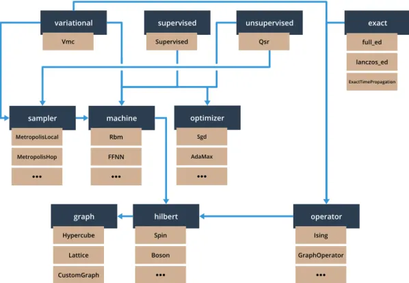
contain some additional functionality for output and statistics that is used internally in other parts of NetKet.

An overview of the most important modules and their de-pendencies is given inFig. 1. A more detailed description of the module contents will be given in the next section.

NetKet uses the Eigen 3 library [19] for linear algebra routines. In the Python interface, Eigen datatypes are transparently con-verted to and from NumPy [20] arrays by

pybind11

. The NetKet driver classes provide methods to directly write the simulation output to JSON files, which is done with the help of the

nlohman-n/json

library for C++ [21]. Parallelization is implemented based on the Message Passing Interface (MPI), allowing to substantially decrease running time. Specifically, the Monte Carlo sampling of expectation values implemented in the

variational.Vmc

class is parallelized, with each node drawing independent samples from the probability distribution which are averaged over all nodes.

2.2. Software functionalities

The core feature of NetKet is the variational representation of quantum states by artificial neural networks. Given a variational state, the task is to optimize its parameters with regard to a specified loss function, such as the total energy for ground state searches or the (negative) overlap with a given target state. In this section, we will discuss the models, types of variational wavefunctions, and learning schemes that are available in NetKet.

2.2.1. Model specification

NetKet currently supports lattice models with a finite Hilbert space of the formH

=

H⊗_localN where N denotes the number of lattice sites andH_local denotes the local Hilbert space of each site. The system is defined on a graph with a set ofN sites and a set of edges (also called bonds) between pairs of sites. This graph structure is used to help with the definition of operators on the lattice and to encode the spatial structure of the model, which is necessary, e.g., to work with convolutional neural net-works (CNNs). NetKet provides the predefined

Hypercube

and

Lattice

graphs. Furthermore,

CustomGraph

supports arbitrary edge-colored graphs, where each edge is associated with an in-teger label called its color. This color can be used to describe different types of bonds.

General lattice spin models can be described straightforwardly in this manner. Bosonic lattice models can also be easily rep-resented by truncating the local Hilbert space to only allow for

Fig. 1. The main submodules of thenetket Python module and their dependencies from a user perspective (i.e., only dependencies in the public interface are shown). Below each submodule, examples of contained classes and functions are displayed. In a typical workflow, users will first define a quantum model, specify a variational representation of the wavefunction as well as the Monte Carlo sampling and optimization methods, and then run the simulation using one of the driver classes. A more detailed description of the software architecture and features is given in the main text.

occupations of up toNlocalbosons per site [22]. NetKet currently provides pre-defined Hamiltonians for the transverse-field Ising, Heisenberg, and Bose–Hubbard models. Other observables and custom Hamiltonians can also be specified: a convenient option for common lattice models is to use the

GraphOperator

class, which allows to construct a Hamiltonian from a family of 2-local operators acting on each bond of a selected color and a family of 1-local operators acting on each site. It is also possible to specify generalk-local operators (as well as their products and sums) using the

LocalOperator

class.

While fermionic Hamiltonians are not fully supported in the present version, they can be implemented using a custom Jordan– Wigner mapping and the

LocalOperator

class [23].

2.2.2. Variational quantum states

The purpose of variational states is to provide a compact and computationally efficient representation of quantum states. Since generally only a subset of the full many-body Hilbert space will be covered by a given variational ansatz, the aim is to use a parametrization that captures the relevant physical states for a given problem.

The variational wavefunctions supported by NetKet are pro-vided as part of the

machine

module, which currently includes NQS but also Jastrow wavefunctions [24,25] and matrix-product states (MPS) [26–28].

Broadly, there are two main types of NQS available in NetKet: restricted Boltzmann machines (RBM) [29] and feed-forward neu-ral networks (FFNN) [8,9,30,31]. Both types of networks are fully complex, i.e., with both complex-valued parameters and output.

The

machine

module contains the

RbmSpin

class for spin-1

2 systems as well as two other variants: the symmetric RBM (

RbmSpinSymm

) to capture lattice symmetries such as translation

and inversion symmetries and the multi-valued RBM

(

RbmMultiVal

) for systems with larger local Hilbert spaces (such as higher spins or bosonic systems).

FFNNs represent a broad and flexible class of networks and are implemented by the

FFNN

class. They consist of a sequence of lay-ers available from the

layer

submodule, each layer performing either an affine transformation to the input vector or applying a non-linear activation function. There are currently two types of affine maps available:

•

Dense fully-connected layers, which for an inputx

∈

_Cn_and outputy

∈

_Cmhave the formy

=

Wx

+

bwhereW

∈

_Cm×n and b

∈

_Cm _{are called theweight matrix and bias vector,} respectively.

•

Convolutional layers [30,32] for hypercubic lattices. As activation functions, rectified linear units (

Relu

) [33], hy-perbolic tangent (

Tanh

) [34], and the logarithm of the hyper-bolic cosine (

Lncosh

) are provided. RBMs without visible bias can be represented as single-layer FFNNs with ln cosh activa-tion, allowing for a generalization of these machines to multiple layers [5].

The

machine

module also provides more traditional varia-tional wavefunctions, namely MPS with periodic boundary con-ditions (

MPSPeriodic

) and long-range Jastrow (

Jastrow

) wave-functions, which allows for comparison of NQS with results ob-tained using these approaches.

Finally, NetKet also includes representations of mixed states in the

machine.densitymatrix

submodule, which most no-tably includes the real-valued NDO ansatz (

NdmSpinPhase

). For compatibility with the rest of the package, the vectorized repre-sentation of density matrices can be accessed through the same interface as NQS.

Custom wavefunctions may be provided by implementing sub-classes of the

AbstractMachine

class in C++ or in Python by deriving

netket.machine.CxxMachine

.

In supervised learning, a target wavefunction is given and the task is to optimize a chosen ansatz to represent it. This functionality is contained within the

supervised

module. Given a variational state

|

Ψ_NN(

α

)

⟩

depending on the parameters

α

∈

_Cm and a target state

|

Ψ_tar

⟩

, the negative log overlap

L(

α

)

= −

log

⟨

Ψtar

|

ΨNN(

α

)

⟩

⟨

Ψ_tar

|

Ψ_tar

⟩

⟨

Ψ_NN(

α

)

|

Ψ_tar

⟩

⟨

Ψ_NN(

α

)

|

Ψ_NN(

α

)

⟩

(1)

is taken as the loss function to be minimized. The loss is com-puted in a Monte Carlo fashion by direct sampling of the target wavefunction. To minimize the loss, the gradient

∇

_αL of the loss function with respect to the parameters is calculated. This gradient is then used to update the parameters according to a specified gradient-based optimization scheme. For example, in stochastic gradient descent (SGD) the parameters are updated as

α

→

α

−

λ

∇

_αL (2)

where

λ

is the learning rate. The different update rules supported by NetKet are contained in the

optimizer

module. Various types of optimizers are available, including SGD, AdaGrad [35], AdaMax and AdaDelta [36], AMSGrad [37], and RMSProp.

2.2.4. Unsupervised learning

NetKet also allows to carry out unsupervised learning of un-known probability distributions, which in this context corre-sponds to quantum state tomography [38]. Given an unknown quantum state, a neural network can be trained on projective measurement data to discover an approximate reconstruction of the state [4]. In NetKet, this functionality is contained within the

unsupervised.Qsr

class.

For some given target quantum state

|

Ψ_tar

⟩

, the training dataset D consists of a sequence of projective measurements

σ

b _{in different bases b, with underlying probability distribution} P(

σ

b₎

_{= |}

_Ψ

tar(

σ

b)

|

2

. The quantum reconstruction of the target state translates into minimizing the statistical divergence be-tween the distribution of the measurement outcomes and the distribution generated by the NQS. This corresponds, up to a constant dataset entropy contribution, to maximizing the log-likelihood of the network distribution over the measurement data

L

=

∑

σb∈D

log

π

(

σ

b)

,

(3)

where

π

denotes the probability distribution

π

(

σ

)

=

|

ΨNN(

σ

)

|

2

∑

σ′

|

Ψ_NN(

σ

′)

|

2

.

(4)

generated by the NQS wavefunction.

Note that, for every training sample where the measurement basis differs from the reference basis

|

σ

⟩

of the NQS, a unitary transformationU

ˆ

should be applied to appropriately change the basis,ΨNN(

σ

b)

= ˆ

UbΨNN(

σ

).

The network parameters are updated according to the gradient of the log-likelihoodL. This can be computed analytically, and it requires expectation values over both the training data points and the network distribution

π

(

σ

). While the first is trivial to compute, the latter should be approximated by a Monte Carlo average over configurations sampled from a Markov chain.

2.2.5. Variational Monte Carlo

Finally, NetKet supports ground state searches for a given many-body quantum HamiltonianH

ˆ

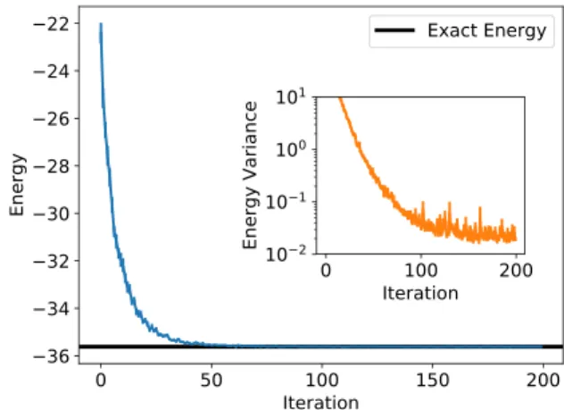
. In this context, the task is to optimize the parameters of a variational wavefunctionΨ in order

Fig. 2.Variational optimization of the restricted Boltzmann machine for the one-dimensional spin-1

2 Heisenberg model. The main plot shows the Monte

Carlo energy estimate, which converges to the exact ground state energy up to a relative error|(E−Eexact)/Eexact|of 4.16×10−5 _{within the 200 iteration}

steps shown. The inset shows the Monte Carlo estimate of the energy variance, which becomes zero in an exact eigenstate of the Hamiltonian.

to minimize the energy

⟨ ˆ

H

⟩

. The

variational.Vmc

driver class contains the main logic to optimize a variational wavefunction given a Hamiltonian, a sampler, and an optimizer.

The energy of a wavefunctionΨ(

σ

)

= ⟨

σ

|

Ψ

⟩

can be estimated as

⟨ ˆ

H

⟩ =

∑

σ,σ′Ψ∗(

σ

)

⟨

σ

| ˆ

H

|

σ

′

⟩

Ψ(

σ

′)

∑

σ

|

Ψ(

σ

)

|

2

=

∑

σ

(

∑

σ′

⟨

σ

| ˆ

H

|

σ

′

⟩

Ψ(

σ

′ ) Ψ(

σ

)

)

|

Ψ(

σ

)

|

2

∑

σ′

|

Ψ(

σ

′)

|

2

≈

⟨

∑

σ′

⟨

σ

| ˆ

H

|

σ

′

⟩

Ψ(

σ

′ ) Ψ(

σ

)

⟩

σ (5)

where in the last line

⟨ · ⟩

_σdenotes a stochastic expectation value taken over a sample of configurations

{

σ

}

drawn from the proba-bility distribution corresponding to the variational wavefunction

(4). This sampling is performed by classes from the

sampler

module, which generate Markov chains of configurations using the Metropolis algorithm [39] to ensure detailed balance. Parallel tempering [40] options are also available to improve sampling efficiency.

In order to optimize the parameters of a machine to minimize the energy, a gradient-based optimization scheme can be applied as discussed in the previous section. The energy gradient can be estimated at the same time as

⟨ ˆ

H

⟩

[2,25]. This requires computing the partial derivatives of the wavefunction with respect to the variational parameters, which can be obtained analytically for the RBM [2] or via backpropagation [30,31,34] for multi-layer FFNNs. In this case, the steepest descent update according to Eq.(2) is also a form of SGD, because the energy is estimated using a sub-set of the full data available from the variational wavefunction. Alternatively, often more stable convergence can be achieved by using the stochastic reconfiguration (SR) method [41,42], which approximates the imaginary time evolution of the system on the submanifold of variational states. The SR approach is closely related to the natural gradient descent method used in machine learning [43]. In the NetKet implementation, SR is performed using either an exact or an iterative linear solver, the latter being recommended when the number of variational parameters is large.

Information on the optimization run (sampler acceptance rates, energy, energy variance, expectation of additional observ-ables, and the current variational parameters) for each iteration

1 import netket as nk 2

3 # Define the graph : a 1D chain o f 20 s i t e s with p e r i o d i c

4 # boundary c o n d i t i o n s

5 g = nk . graph . Hypercube ( length =20 , n_dim =1 , pbc=True ) 6

7 # Define the H i l b e r t Space : spin h a l f degree o f freedom a t each

8 # s i t e o f the graph , r e s t r i c t e d to the zero magnetization s e c t o r

9 h i = nk . h i l b e r t . Spin ( s = 0 . 5 , t o t a l _ s z = 0 . 0 , graph=g ) 10

11 # Define the Hamiltonian : spin h a l f Heisenberg model

12 ha = nk . operator . Heisenberg ( h i l b e r t = h i ) 13

14 # Define the ansatz : R e s t r i c t e d Boltzmann machine

15 # with 20 hidden u n i t s

16 ma = nk . machine . RbmSpin ( h i l b e r t = hi , n_hidden =20) 17

18 # I n i t i a l i s e with machine parameters

19 ma . init_random_parameters ( seed =1234 , sigma = 0 . 0 1 ) 20

21 # Define the Sampler : metropolis sampler with l o c a l

22 # exchange moves , i . e . n e a r e s t neighbour spin swaps

23 # which preserve the t o t a l magnetization

24 sa = nk . sampler . MetropolisExchange ( graph=g , machine=ma) 25

26 # Define the optimiser : S t o c h a s t i c g r a d i e n t descent with

27 # l e a r n i n g r a t e 0 . 0 1 .

28 opt = nk . optimizer . Sgd ( l e a r n i n g _ r a t e = 0 . 0 1 ) 29

30 # Define the VMC o b j e c t : S t o c h a s t i c R e c o n f i g u r a t i o n " Sr " i s used

31 gs = nk . v a r i a t i o n a l . Vmc( hamiltonian =ha , sampler=sa ,

32 optimizer =opt , n_samples =1000 ,

33 u s e _ i t e r a t i v e =True , method=’ Sr ’) 34

35 # Run the VMC simulation f o r 1000 i t e r a t i o n s

36 # and save the output i n t o f i l e s with p r e f i x " t e s t "

37 # The machine parameters are s to r ed i n " t e s t . wf"

38 # while the measurements are s to r ed i n " t e s t . l o g "

39 gs . run ( o u t p u t _ p r e f i x =’ t e s t ’, n _ i t e r =1000)

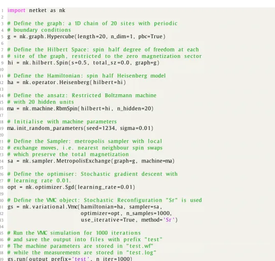
Listing 1: Example script for finding the ground state of the one-dimensional spin-1₂ Heisenberg model using an RBM ansatz.

can be written to a log file in JSON format. Alternatively, they can be accessed directly inside the simulation loop in Python to allow for more flexible output.

3. Illustrative examples

NetKet is available as a Python package and can be obtained from the Python package index (PyPI) [44]. Assuming a properly configured Python environment, NetKet can be installed via the shell command

pip install netket

which will download, compile, and install the package. A working MPI environment is required to run NetKet. In case multiple MPI installations are present on the system and in order to avoid po-tential conflicts, we recommend to run the installation command as

CC=mpicc CXX=mpicxx pip install netket

with the desired MPI environment loaded in order to perform the build with the correct compiler. After a successful installation, the NetKet module can be imported in Python scripts.

Alternatively to installing NetKet locally, NetKet also uses the deployment of BinderHub from mybinder.org [45] to build and deploy a stable version of the software, which can be found at

https://mybinder.org/v2/gh/netket/netket/v.2.0. This allows users to run the tutorials or other small jobs without installing NetKet.

Fig. 3. Supervised learning of the ground state of the one-dimensional spin-1₂ transverse field Ising model with 10 sites from ED data, using an RBM with 20 hidden units. The blue line shows the overlap between the RBM wavefunction and the exact wavefunction for each iteration.

3.1. One-dimensional Heisenberg model

As a first example, we present a Python script for obtaining a variational RBM representation of the ground state of the

spin-1

2 Heisenberg model on a one-dimensional chain with periodic boundary conditions. The code for this example is shown in Listing 1. Fig. 2 shows the evolution of the energy expectation value over the course of the optimization run. We see that for a small chain of 20 sites and an RBM with 20 hidden units, the

1 import netket as nk 2 from numpy import l o g 3

4 # 1D L a t t i c e

5 g = nk . graph . Hypercube ( length =10 , n_dim =1 , pbc=True ) 6

7 # H i l b e r t space o f s p i n s on the graph

8 h i = nk . h i l b e r t . Spin ( s = 0 . 5 , graph=g ) 9

10 # I s i n g spin Hamiltonian

11 ha = nk . operator . I s i n g ( h = 1 . 0 , h i l b e r t = h i ) 12

13 # Perform Exact D i a g o n a l i z a t i o n to get lowest e i g e n v e c t o r

14 r e s = nk . exact . lanczos_ed ( ha , f i r s t _ n =1 , compute_eigenvectors =True ) 15

16 # S t o r e e i g e n v e c t o r as a l i s t o f t r a i n i n g samples and t a r g e t s

17 # The samples would be the H i l b e r t space c o n f i g u r a t i o n s and

18 # the t a r g e t s should be wavefunction amplitudes .

19 hind = nk . h i l b e r t . H i l b e r t I n d e x ( h i ) 20 h _ s i z e = hind . n _ s t a t e s

21 t a r g e t s = [ [ l o g ( r e s . e i g e n v e c t o r s [ 0 ] [ i ] ) ] f o r i i n range( h _ s i z e ) ] 22 samples = [ hind . number_to_state ( i ) f o r i i n range( h _ s i z e ) ] 23

24 # Machine : R e s t r i c t e d Boltzmann machine

25 # with 20 hidden u n i t s

26 ma = nk . machine . RbmSpin ( h i l b e r t = hi , n_hidden =20) 27 ma . init_random_parameters ( seed =1234 , sigma = 0 . 0 1 ) 28

29 # Optimizer

30 op = nk . optimizer . AdaMax ( ) 31

32 # Supervised Learning module

33 spvsd = nk . supervised . Supervised ( machine=ma,

34 optimizer =op , 35 b a t c h _ s i z e =400 , 36 samples=samples , 37 t a r g e t s = t a r g e t s ) 38 39 # Run the o p t i m i za t i o n f o r 2000 i t e r a t i o n s 40 spvsd . run ( n _ i t e r =2000 , o u t p u t _ p r e f i x =’ t e s t ’, 41 l o s s _ f u n c t i o n =" Overlap_phi ")

Listing 2: Example script for supervised learning. A RBM ansatz is optimized to represent the ground state of the one-dimensional spin-1

2 transverse field Ising model obtained by ED for this example.

energy converges to a relative error of the order 10−5 within about 100 iteration steps.

3.2. Supervised learning

As a second example, we use the supervised learning module in NetKet to optimize an RBM to represent the ground state of the transverse field Ising model. The example script is shown in Listing2. The exact ground state wavefunction is first obtained by exact diagonalization and then used for training the RBM state by minimizing the overlap loss(1).Fig. 3shows the evolution of the overlap over the training iterations.

4. Impact

Given the flexibility of NetKet, we envision several poten-tial applications of this library both in data-driven experimental research and in more theoretical, problem-driven research on interacting quantum many-body systems. For example, several important theoretical and practical questions concerning the ex-pressibility of NQS, the learnability of experimental quantum states, and the efficiency at finding ground states ofk-local Hamil-tonians, can be directly addressed using the current functionality of the software.

Moreover, having an easy-to-extend set of tools to work with NQS-based applications can propel future research in the field, without researchers having to pay a significant cost of entry in

terms of algorithm implementation and testing. Since its early release in April 2017, NetKet has already been used for research purposes by several groups worldwide [5,22,23,46–48]. We also hope that, building upon a common set of tools, practices like publishing accompanying codes to research papers, largely pop-ular in the ML community, can become standard practice also for ML applications in quantum physics.

Finally, for a fast-growing community like ML for quantum science, it is also crucial to have pedagogical tools available that can be conveniently used by new generations of students and researchers. Benefiting from a growing set of tutorials and step-by-step explanations, NetKet can be comfortably used in schools and lectures.

5. Conclusions and future directions

We have introduced NetKet, a comprehensive open source framework for the study of many-body quantum systems us-ing machine learnus-ing techniques. Central to this framework are variational parameterizations of many-body wavefunctions in the form of artificial neural networks. NetKet is a Python framework implemented in C++11, designed with efficiency as well as ease of use in mind. Several examples, tutorials, and notebooks are provided with our software in order to reduce the learning curve for newcomers.

The NetKet project is meant to continuously evolve in fu-ture releases, welcoming suggestions and contributions from its users. For example, future versions may provide a natural in-terface with general ML frameworks such as PyTorch [49] and Tensorflow [50]. On the algorithmic side, future goals include the extension of NetKet to incorporate unitary dynamics [11,

51], convenient Fermionic operators, as well as full support for density-matrix tomography [17].

Declaration of competing interest

The authors declare that they have no known competing finan-cial interests or personal relationships that could have appeared to influence the work reported in this paper.

Acknowledgments

We acknowledge support from the Flatiron Institute of the Simons Foundation. J.E.T.S. gratefully acknowledges support from a fellowship through The Molecular Sciences Software Institute under NSF Grant ACI1547580. H.T. is supported by a grant from the Fondation CFM pour la Recherche. S.E. and I.G. are supported by an ERC Advanced Grant QENOCOBA under the EU Horizon2020 program (grant agreement 742102) and the German Research Foundation (DFG) under Germany’s Excellence Strategy through Project No. EXC-2111 - 390814868 (MCQST).

This project makes use of other open source software, namely pybind11 [16], Eigen [19], nlohmann/json [21], NumPy [20], and SciPy [18].

Pre-release versions of NetKet 2.0 have used a Lanczos solver based on the IETL library from the ALPS project [52,53], which implements a variant of the Lanczos algorithm due to Cullum and Willoughby [54,55].

We further acknowledge discussions with, as well as bug reports, comments, and support from S. Arnold, A. Booth, A. Borin, J. Carrasquilla, C. Ciuti, S. Lederer, Y. Levine, T. Neupert, O. Par-collet, A. Rubio, M. A. Sentef, O. Sharir, M. Stoudenmire, and N. Wies.

References

[1] Carleo G, Cirac I, Cranmer K, Daudet L, Schuld M, Tishby N, Vogt-Maranto L, Zdeborová L. Machine learning and the physical sciences. 2019, arXiv: 1903.10563.

[2] Carleo G, Troyer M. Solving the quantum many-body problem with ar-tificial neural networks. Science 2017;355(6325):602–6.http://dx.doi.org/ 10.1126/science.aag2302, URL http://science.sciencemag.org/content/355/ 6325/602.

[3] Cai Z, Liu J. Approximating quantum many-body wave functions using arti-ficial neural networks. Phys Rev B 2018;97(3):035116.http://dx.doi.org/10. 1103/PhysRevB.97.035116, URL https://link.aps.org/doi/10.1103/PhysRevB. 97.035116.

[4] Torlai G, Mazzola G, Carrasquilla J, Troyer M, Melko R, Carleo G. Neural-network quantum state tomography. Nat Phys 2018;14(5):447– 50. http://dx.doi.org/10.1038/s41567-018-0048-5, URL https://doi.org/10. 1038/s41567-018-0048-5.

[5] Choo K, Carleo G, Regnault N, Neupert T. Symmetries and many-body excitations with neural-network quantum states. Phys Rev Lett 2018;121:167204. http://dx.doi.org/10.1103/PhysRevLett.121.167204, URL

https://link.aps.org/doi/10.1103/PhysRevLett.121.167204.

[6] Glasser I, Pancotti N, August M, Rodriguez ID, Cirac JI. Neural-network quantum states, string-bond states, and chiral topological states. Phys. Rev. X 2018;8:011006.http://dx.doi.org/10.1103/PhysRevX.8.011006, URL

https://link.aps.org/doi/10.1103/PhysRevX.8.011006.

[7] Kaubruegger R, Pastori L, Budich JC. Chiral topological phases from arti-ficial neural networks. Phys. Rev. B 2018;97:195136.http://dx.doi.org/10. 1103/PhysRevB.97.195136, URL https://link.aps.org/doi/10.1103/PhysRevB. 97.195136.

[8] Saito H. Solving the bose-hubbard model with machine learning. J Phys Soc Japan 2017;86(9):093001.http://dx.doi.org/10.7566/JPSJ.86.093001.

[9] Saito H, Kato M. Machine learning technique to find quantum many-body ground states of bosons on a lattice. J Phys Soc Japan 2018;87(1):014001.

http://dx.doi.org/10.7566/JPSJ.87.014001.

[10] Czischek S, Gärttner M, Gasenzer T. Quenches near ising quantum criticality as a challenge for artificial neural networks. Phys. Rev. B 2018;98:024311. http://dx.doi.org/10.1103/PhysRevB.98.024311, URL

https://link.aps.org/doi/10.1103/PhysRevB.98.024311.

[11] Jónsson B, Bauer B, Carleo G. Neural-network states for the classical simulation of quantum computing. 2018, arXiv:1808.05232, URL http: //arxiv.org/abs/1808.05232.

[12] Hartmann MJ, Carleo G. Neural-network approach to dissipative quan-tum many-body dynamics. Phys Rev Lett 2019;122:250502.http://dx.doi. org/10.1103/PhysRevLett.122.250502, URLhttps://link.aps.org/doi/10.1103/ PhysRevLett.122.250502.

[13] Yoshioka N, Hamazaki R. Constructing neural stationary states for open quantum many-body systems. Phys Rev B 2019;99(21):214306.http://dx. doi.org/10.1103/PhysRevB.99.214306, URLhttps://link.aps.org/doi/10.1103/ PhysRevB.99.214306.

[14] Nagy A, Savona V. Variational quantum monte carlo method with a neural-network ansatz for open quantum systems. Phys Rev Lett 2019;122(25):250501. http://dx.doi.org/10.1103/PhysRevLett.122.250501, URLhttps://link.aps.org/doi/10.1103/PhysRevLett.122.250501.

[15] Vicentini F, Biella A, Regnault N, Ciuti C. Variational neural-network ansatz for steady states in open quantum systems. Phys Rev Lett 2019;122(25):250503. http://dx.doi.org/10.1103/PhysRevLett.122.250503, URLhttps://link.aps.org/doi/10.1103/PhysRevLett.122.250503.

[16] Jakob W, Rhinelander J, Moldovan D. Pybind11 – seamless operability between c++11 and python. 2019.

[17] Torlai G, Melko RG. Latent space purification via neural density operators. Phys Rev Lett 2018;120(24):240503.http://dx.doi.org/10.1103/PhysRevLett. 120.240503, URLhttps://link.aps.org/doi/10.1103/PhysRevLett.120.240503. [18] Jones E, Oliphant T, Peterson P, et al. SciPy: Open source scientific tools for Python. 2001, URLhttp://www.scipy.org/. [Online; Accessed 5 July 2019]. [19] Guennebaud G, Jacob B, et al. Eigen v3. 2010.

[20] Oliphant T. NumPy: A Guide to NumPy. USA: Trelgol Publishing; 2006, URL

https://www.numpy.org/.

[21] Lohmann N, et al. JSON for modern C++. GitHub Repository 2019.

[22] McBrian K, Carleo G, Khatami E. Ground state phase diagram of the one-dimensional bose-Hubbard model from restricted Boltzmann machines.

arXiv:1903.03076.

[23] Choo K, Mezzacapo A, Carleo G. Quantum Chemistry with Neural-Network Quantum States [in preparation].

[24] Manousakis E. The spin-1

2 heisenberg antiferromagnet on a square lattice

and its application to the cuprous oxides. Rev Modern Phys 1991;63:1– 62. http://dx.doi.org/10.1103/RevModPhys.63.1, URL https://link.aps.org/ doi/10.1103/RevModPhys.63.1.

[25] Becca F, Sorella S. Quantum Monte Carlo Approaches for Correlated Systems. first ed. Cambridge University Press; 2017,http://dx.doi.org/10. 1017/9781316417041.

[26] White SR. Density matrix formulation for quantum renormalization groups. Phys Rev Lett 1992;69(19):2863–6.http://dx.doi.org/10.1103/physrevlett. 69.2863.

[27] Rommer S, Östlund S. Class of ansatz wave functions for one-dimensional spin systems and their relation to the density matrix renormaliza-tion group. Phys Rev B 1997;55(4):2164–81. http://dx.doi.org/10.1103/ physrevb.55.2164.

[28] Schollwöck U. The density-matrix renormalization group in the age of matrix product states. Ann Physics 2011;326(1):96–192.http://dx.doi.org/ 10.1016/j.aop.2010.09.012.

[29] Hinton GE. Reducing the dimensionality of data with neural networks. Science 2006;313(5786):504–7.http://dx.doi.org/10.1126/science.1127647. [30] LeCun Y, Bengio Y, Hinton GE. Deep learning. Nature 2015;521(7553):436–

44.http://dx.doi.org/10.1038/nature14539.

[31] Goodfellow I, Bengio Y, Courville A. Deep Learning. MIT Press; 2016.

[32] Gu J, Wang Z, Kuen J, Ma L, Shahroudy A, Shuai B, Liu T, Wang X, Wang G, Cai J, Chen T. Recent advances in convolutional neural networks. Pattern Recognit 2018;77:354–77. http://dx.doi.org/10.1016/j.patcog.2017.10.013, URLhttp://www.sciencedirect.com/science/article/pii/S0031320317304120. [33] Nair V, Hinton GE. Rectified linear units improve restricted Boltzmann machines. In: Proceedings of the 27th international conference on machine learning. 2010. p. 807–14. URLhttp://www.icml2010.org/papers/432.pdf. [34] LeCun Y, Bottou L, Orr GB, Müller K. Efficient BackProp. In: Neural

Networks: Tricks of the Trade. second ed.. 2012, p. 9–48.http://dx.doi. org/10.1007/978-3-642-35289-8_3.

[35] Duchi J, Hazan E, Singer Y. Adaptive subgradient methods for online learning and stochastic optimization. J Mach Learn Res 2011;12(Jul):2121– 59.

[36] Kingma DP, Ba J. Adam: A method for stochastic optimization. 2014, CoRR abs/1412.6980.arXiv:1412.6980, URLhttp://arxiv.org/abs/1412.6980.

In: International conference on learning representations. 2018. URLhttps: //openreview.net/forum?id=ryQu7f-RZ.

[38] James DFV, Kwiat PG, Munro WJ, White AG. Measurement of qubits. Phys. Rev. A 2001;64:052312. http://dx.doi.org/10.1103/PhysRevA.64.052312, URLhttps://link.aps.org/doi/10.1103/PhysRevA.64.052312.

[39] Metropolis N, Rosenbluth AW, Rosenbluth MN, Teller AH, Teller E. Equa-tion of state calculaEqua-tions by fast computing machines. J Chem Phys 1953;21(6):1087–92.http://dx.doi.org/10.1063/1.1699114.

[40] Swendsen RH, Wang J-S. Replica Monte Carlo simulation of spin-glasses. Phys Rev Lett 1986;57:2607–9. http://dx.doi.org/10.1103/PhysRevLett.57. 2607, URLhttps://link.aps.org/doi/10.1103/PhysRevLett.57.2607.

[41] Sorella S. Green function Monte Carlo with stochastic reconfiguration. Phys Rev Lett 1998;80:4558–61.http://dx.doi.org/10.1103/PhysRevLett.80.4558, URLhttps://link.aps.org/doi/10.1103/PhysRevLett.80.4558.

[42] Casula M, Sorella S. Geminal wave functions with Jastrow correlation: A first application to atoms. J Chem Phys 2003;119(13):6500–11. http: //dx.doi.org/10.1063/1.1604379.

[43] Amari S-i. Natural gradient works efficiently in learning. Neural Comput 1998;10(2):251–76.http://dx.doi.org/10.1162/089976698300017746. [44] PyPI – the Python package index. https://pypi.org/. [Accessed 6 March

2019].

[45] Jupyter P, Bussonnier M, Forde J, Freeman J, Granger B, Head T, Holdgraf C, Kelley K, Nalvarte G, Osheroff A, Pacer M, Panda Y, Perez F, Ragan-Kelley B, Willing C. Binder 2.0 - Reproducible, interactive, sharable environments for science at scale. In: Fatih Akici and David Lippa and Dillon Niederhut and M Pacer, editors, Proceedings of the 17th python in science conference. 2018. p. 113–20.http://dx.doi.org/10.25080/Majora-4af1f417-011. [46] Choo K, Neupert T, Carleo G. Study of the two-dimensional frustrated

J1-J2 model with neural network quantum states.arXiv:1903.06713. URL

http://arxiv.org/abs/1903.06713.

[47] Vieijra T, Casert C, Nys J, De Neve W, Haegeman J, Ryckebusch J, Verstraete F. Restricted Boltzmann machines for quantum states with nonabelian or anyonic symmetries.arXiv:1905.06034. URLhttp://arxiv.org/ abs/1905.06034.

[48] Pilati S, Inack EM, Pieri P. Self-learning projective quantum Monte Carlo simulations guided by restricted Boltzmann machines.arXiv:1903.00907. URLhttp://arxiv.org/abs/1907.00907.

Desmaison A, Antiga L, Lerer A. Automatic differentiation in PyTorch. In: NIPS-W. 2017.

[50] Abadi M, Agarwal A, Barham P, Brevdo E, Chen Z, Citro C, Corrado GS, Davis A, Dean J, Devin M, Ghemawat S, Goodfellow I, Harp A, Irving G, Isard M, Jia Y, Jozefowicz R, Kaiser L, Kudlur M, Levenberg J, Mané D, Monga R, Moore S, Murray D, Olah C, Schuster M, Shlens J, Steiner B, Sutskever I, Talwar K, Tucker P, Vanhoucke V, Vasudevan V, Viégas F, Vinyals O, Warden P, Wattenberg M, Wicke M, Yu Y, Zheng X. TensorFlow: Large-scale machine learning on heterogeneous systems. 2015, Software available from . URLhttp://tensorflow.org/.

[51] Carleo G, Becca F, Schiro M, Fabrizio M. Localization and glassy dynamics of many-body quantum systems. Sci Rep 2012;2:243.http://dx.doi.org/10. 1038/srep00243.

[52] Bauer B, Carr LD, Evertz HG, Feiguin A, Freire J, Fuchs S, Gamper L, Gukelberger J, Gull E, Guertler S, Hehn A, Igarashi R, Isakov SV, Koop D, Ma PN, Mates P, Matsuo H, Parcollet O, Pawłowski G, Picon JD, Pollet L, Santos E, Scarola VW, Schollwöck U, Silva C, Surer B, Todo S, Trebst S, Troyer M, Wall ML, Werner P, Wessel S. The ALPS project release 2.0: open source software for strongly correlated systems. J Stat Mech Theory Exp 2011;2011(05):P05001.http://dx.doi.org/10.1088/1742-5468/2011/05/ p05001, URLhttps://doi.org/10.1088/1742-5468/2011/05/p05001. [53] Albuquerque A, Alet F, Corboz P, Dayal P, Feiguin A, Fuchs S, Gamper L,

Gull E, Gürtler S, Honecker A, Igarashi R, Körner M, Kozhevnikov A, Läuchli A, Manmana S, Matsumoto M, McCulloch I, Michel F, Noack R, Pawłowski G, Pollet L, Pruschke T, Schollwöck U, Todo S, Trebst S, Troyer M, Werner P, Wessel S. The ALPS project release 1.3: Open-source software for strongly correlated systems. J Magn Magn Mater 2007;310(2):1187–93. http://dx.doi.org/10.1016/j.jmmm.2006.10.304, URL

https://doi.org/10.1016/j.jmmm.2006.10.304.

[54] Cullum J, Willoughby RA. Computing eigenvalues of very large symmetric matrices—An implementation of a lanczos algorithm with no reorthogonal-ization. J Comput Phys 1981;44(2):329–58. http://dx.doi.org/10.1016/0021-9991(81)90056-5.

[55] Cullum J, Willoughby RA. Lanczos Algorithms for Large Symmetric Eigen-value Computations Vol. I Theory (Progress in Scientific Computing) (Volume 1). Birkhäuser; 1985.