Research Article
Improving Vector Evaluated Particle Swarm Optimisation Using
Multiple Nondominated Leaders
Kian Sheng Lim,
1Salinda Buyamin,
1Anita Ahmad,
1Mohd Ibrahim Shapiai,
1Faradila Naim,
2Marizan Mubin,
3and Dong Hwa Kim
41Faculty of Electrical Engineering, Universiti Teknologi Malaysia, 81310 Johor Bahru, Malaysia 2Faculty of Electrical & Electronic Engineering, Universiti Malaysia Pahang, 26600 Pekan, Malaysia
3Department of Electrical Engineering, Faculty of Engineering, Universiti Malaya, 50603 Kuala Lumpur, Malaysia 4Department of Instrumentation and Control Engineering, Hanbat National University, Daejeon 305-719, Republic of Korea Correspondence should be addressed to Faradila Naim; [email protected]
Received 10 February 2014; Accepted 9 March 2014; Published 27 April 2014 Academic Editors: P. Agarwal, V. Bhatnagar, and Y. Zhang
Copyright © 2014 Kian Sheng Lim et al. This is an open access article distributed under the Creative Commons Attribution License, which permits unrestricted use, distribution, and reproduction in any medium, provided the original work is properly cited. The vector evaluated particle swarm optimisation (VEPSO) algorithm was previously improved by incorporating nondominated solutions for solving multiobjective optimisation problems. However, the obtained solutions did not converge close to the Pareto front and also did not distribute evenly over the Pareto front. Therefore, in this study, the concept of multiple nondominated leaders is incorporated to further improve the VEPSO algorithm. Hence, multiple nondominated solutions that are best at a respective objective function are used to guide particles in finding optimal solutions. The improved VEPSO is measured by the number of nondominated solutions found, generational distance, spread, and hypervolume. The results from the conducted experiments show that the proposed VEPSO significantly improved the existing VEPSO algorithms.
1. Introduction
Multiobjective optimisation (MOO) problems involve the simultaneous minimisation/maximisation of multiple objec-tive functions, which usually conflict with each other. Due to the conflict between objective functions, a single solu-tion could not satisfy all objective funcsolu-tions. Hence, MOO problem usually results in a set of tradeoffs or nondominated solutions. The vector evaluated particle swarm optimisation (VEPSO) [1] algorithm has been widely used to solve MOO problems [2–7]. As an example, VEPSO algorithm has been implemented in solving DNA sequence problem by min-imising four objective functions, namely,𝐻measure, similarity,
continuity, and hairpin, and two constraints, namely, melting temperature and GCcontent [7]. Compared to DNA sequence
design using binary particle swarm optimization which produces single set of DNA sequences [8], VEPSO is able to generate several sets of good DNA sequences which fulfil the four objective functions and two constraints.
The VEPSO algorithm is adapted from the vector eval-uated genetic algorithm (VEGA) [9], in which each swarm
optimises one objective function by using the best solution from another swarm as a guidance. However, the VEPSO suf-fers from performance drawback. Therefore, it is improved by redefining the selection of the guidance from nondominated solution, known as VEPSOnds [10]. Although VEPSOnds has shown better performance than conventional VEPSO, the VEPSOnds suffers from weak performance in terms of lacking solution distributions and convergence to the true Pareto front.
Other than VEPSOnds, there are various MOO algo-rithms which used nondominated solution to guide parti-cle in finding the optimum solutions for MOO problem. For example, in Multiobjective particle swarm optimisation (MOPSO) algorithm [11, 12], all nondominated solutions are separated into groups according to their location in the objective space. A guiding solution for each particle is then randomly selected from the group containing the fewest solutions. Besides, in nondominated sorting PSO (NSPSO) algorithm [13], which uses the main mechanism of the nondominated sorting fenetic algorithm-II [14], each particle is guided by a nondominated solution that is randomly
Volume 2014, Article ID 364179, 21 pages http://dx.doi.org/10.1155/2014/364179
selected using the niche count and the nearest neighbour density estimator. A nondominated solution is selected based on binary tournament selection for the purpose of guiding the other particles in the optimised MOPSO (OMOPSO) algorithm [15]. Additionally, Abido [16] introduces the use of two nondominated solutions, which are called the local set and the global set. The guide is selected based on the nearest distance in objective space between each particle and each member of the nondominated solution of both sets.
Noticeably, most particle swarm optimisation- (PSO-) based MOO algorithms, including conventional VEPSO and VEPSOnds, only use one solution as the particle guide. In particular, in VEPSOnds, particles from a swarm will be guided by the nondominated solution which has the best fitness at one objective function. Thus, the particles may guide the searching with limited information about the other objective functions during the optimisation process. Therefore, VEPSOnds can be further improved by using more than one nondominated solution as particle guide. In this context, this improved VEPSO algorithm will use the best solution from all swarms as guidance during the optimisation process.
The next section of this paper explains the particle swarm optimisation (PSO), the conventional VEPSO, VEP-SOnds algorithm, and the proposed VEPSO algorithms. The following section presents the experimental work and the description of the benchmark test problems and performance measures and the discussion of the results. The final section concludes the proposed technique and discusses few possible future works.
2. Multiobjective Optimization
For explanation, consider a minimization problem minimize fitness function,
⃗𝐹 ( ⃗𝑥) = {𝑓𝑖( ⃗𝑥) , 𝑖 = 1, 2, . . . , 𝑀}
subject to= {𝑔𝑗( ⃗𝑥) ≤ 0, 𝑗 = 1, 2, . . . , 𝑝
ℎ𝑘( ⃗𝑥) = 0, 𝑘 = 1, 2, . . . , 𝑞,
(1)
where ⃗𝑥 = {𝑥1, 𝑥2, . . . , 𝑥𝑛} is the decision variable vector which represents the possible solution,𝑀is the number of objectives, and𝑓𝑖 ∈ R𝑛 → Ris the objective function.
{𝑔𝑗, ℎ𝑘} ∈ R𝑛 → Rare the inequality and equality
con-straint function, respectively. The Pareto optimality concept is defined as follows.
Definition 1. Given {→𝐹𝑎,𝐹→𝑏} ∈ R𝑚 as two vectors, →𝐹𝑎
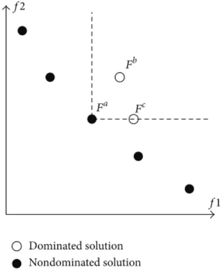
dominates→𝐹𝑏 (denote as→𝐹𝑎 ≺ →𝐹𝑏) if and only if𝑓𝑖𝑎 ≤ 𝑓𝑖𝑏 for𝑖 = 1, 2, . . . , 𝑚and𝑓𝑖𝑎 < 𝑓𝑖𝑏for at least once. Dominance relation of→𝐹𝑎 ≺ →𝐹𝑏 and→𝐹𝑎 ≺ →𝐹𝑐 can be illustrated as the labelled circles inFigure 1for a two-objective problem.
Definition 2. A decision variable vector→𝑥𝑎is anondominated solutionwhen there is no other solution→𝑥𝑏such that ⃗𝐹(→𝑥𝑎) ≺
f2 f1 Dominated solution Fc Fb Fa Nondominated solution
Figure 1: Dominance relation for two-objective problem.
⃗𝐹(→𝑥𝑏). Nondominated solution is also known as Pareto
optimal solution.
Definition 3. The set of nondominated solutions of a MOO problem is known asPareto optimal set,P.
Definition 4. The set of objective vectors with respect toPis known as thePareto front,PF= { ⃗𝐹( ⃗𝑥) ∈R𝑚| ⃗𝑥 ∈P}.PF for a two-objective problem is illustrated as the black circles inFigure 1.
The motivation of MOO is to find as many nondominated solutions as possible according to the objective functions and constraints. However, it is possible to have different solutions which map to the same fitness value in objective space. Therefore, it will be more challenging to find more nondominated solutions.
3. Particle Swarm Optimisation
3.1. Original Particle Swarm Optimisation Algorithm. Particle swarm optimisation (PSO) is a population-based stochastic optimisation algorithm introduced by Kennedy and Eberhart [17]. This algorithm finds an optimal solution using a method inspired by the social behaviour of birds flocking and fish schooling. In the PSO algorithm, an individual is known as a particle, and it holds the possible solution to the optimisation problem, given its position. A particle explores the search space, looking for a better solution with respect to the objective functions defined by the optimisation problem. The search process requires the particle to compare its current position with the best positions that it and the whole swarm have found, so that all particles collaborate with each other.
The PSO algorithm is shown inAlgorithm 1. Consider a minimisation problem in which a swarm of𝐼particles are flying around in an𝑁-dimensional search space, each with a position𝑝𝑖𝑛 (𝑖 = 1, 2, . . . , 𝐼; 𝑛 = 1, 2, . . . , 𝑁)representing the possible solution. At initialization stage, all particles are randomly positioned in the search space with random
begin
Initialiseposition&velocity; Evaluateobjective; InitialisepBest; InitialisegBest (2); while𝑖 ≤ 𝑖maxdo Updatevelocity(3); Updateposition(4); Evaluateobjective; UpdatepBest; UpdategBest (2); 𝑖++; end end
Algorithm 1: The PSO algorithm.
velocity,V𝑖𝑛(𝑡). Subsequently, the objective fitness→𝐹𝑖(𝑡)of each particle is evaluated based on the objective function for𝑝𝑖(𝑡). After that, the particle’s best position, 𝑝Best𝑖(𝑡), is set to its initial position. Additionally, the swarm’s best position,
𝑔Best(𝑡), is the best𝑝Best𝑖(𝑡)among all particles, as in (2), where𝑆is the swarm of particles
𝑔Best= {𝑝Best𝑖∈ 𝑆 | 𝑓 (𝑝Best𝑖) =min𝑓 (∀ 𝑝Best𝑖∈ 𝑆)} . (2) In the search process, the algorithm will iterate until the maximum number of iterations is reached. Within an iteration, the velocity and position of each particle are updated using (3) and (4), respectively,
V𝑖𝑛(𝑡 + 1) = 𝜒 [𝜔V𝑖𝑛(𝑡) + 𝑐1𝑟1(𝑝Best𝑖𝑛− 𝑝𝑛𝑖(𝑡))
+ 𝑐2𝑟2(𝑔Best𝑛− 𝑝𝑛𝑖(𝑡))] ,
(3)
𝑝𝑖𝑛(𝑡 + 1) = 𝑝𝑛𝑖(𝑡) +V𝑖𝑛(𝑡 + 1) , (4) where𝜒is the constriction factor and𝜔is the inertia weight. The𝑟1 and𝑟2are both random numbers ranging from zero to one. The𝑐1and𝑐2are the cognitive and social constants, respectively, which control the attraction of the 𝑝Best𝑖(𝑡) and 𝑔Best(𝑡). Then, the 𝑖⃗𝐹(𝑡) for each particle is evaluated again. After updating the fitness, the new position of particle
𝑖is compared with𝑝Best𝑖(𝑡), and the more optimal of the two is saved as𝑝Best𝑖(𝑡). Next, the 𝑔Best(𝑡) is updated as well with the best among all𝑝Best𝑖(𝑡), as in (2). When the search process ended, the𝑔Best(𝑡)will then represent the best solution found for the problem by this algorithm.
3.2. Vector Evaluated Particle Swarm Optimisation Algorithm.
The VEPSO algorithm, introduced by Parsop´oulos and Vra-hatis [1], uses the multiswarms concept from the VEGA algorithm [9]. Each swarm optimises one objective function using the 𝑔Best(𝑡) from another swarm. In the VEPSO algorithm, the 𝑝Best𝑖(𝑡) which has the best fitness with
respect to the𝑚th objective is the𝑔Best(𝑡)for the𝑚th swarm, as in (5)
𝑔Best𝑚 = {𝑝Best𝑖∈ 𝑆𝑚| 𝑓𝑚(𝑝Best𝑖)
=min𝑓𝑚(∀𝑝Best𝑖∈ 𝑆𝑚)} .
(5)
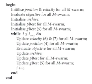
The flow of the VEPSO algorithm is given as in
Algorithm 2. For problem with 𝑀 objective functions, VEPSO algorithm is similar to that of the PSO but some processes are repeated for all𝑀-swarm and nondominated solutions are recorded in an archive. However, the velocity update is reformulated and it is given in (6). Note that the particles in the𝑚th swarm will fly using𝑔Best𝑘(𝑡)where𝑘 is defined by (7). The sharing of𝑔Best(𝑡)between swarms is illustrated inFigure 2: V𝑚𝑛𝑖 (𝑡 + 1) = 𝜒 [𝜔V𝑚𝑖𝑛 (𝑡) + 𝑐1𝑟1(𝑝Best𝑚𝑖𝑛 − 𝑝𝑚𝑖𝑛 (𝑡)) +𝑐2𝑟2(𝑔Best𝑘𝑛− 𝑝𝑚𝑖𝑛 (𝑡))] (6) 𝑘 = {𝑀,𝑚 − 1, 𝑚 = 1 otherwise. (7)
The nondominated solutions are recorded in an archive after the objective functions are evaluated. In the recording process, the fitness→𝐹𝑖(𝑡) of each particle is compared to all others, before it is compared to the nondominated solutions in the archive, using thePareto optimalitycriterion, so that the archive only contains nondominated solutions. At the end of the computation, all nondominated solutions are the possible solutions to the problem.
3.3. The Improved VEPSO Algorithm by Incorporating Non-dominated Solutions. In the search process of conventional VEPSO, as inFigure 3(a), particles from a swarm are opti-mised using the 𝑔Best𝑚(𝑡) from another swarm that has the best fitness at the objective function optimised by the other swarm. However, based on the velocity update of conventional VEPSO in (5), the 𝑔Best𝑚(𝑡) is not updated
begin
Initiliseposition&velocityfor allM-swarm; Evaluateobjectivefor allM-swarm; Initialisearchive;
InitialisepBest for allM-swarm; InitialisegBest (5) for allM-swarm;
while 𝑖 ≤ 𝑖maxdo
Updatevelocity(6) & (7) for allM-swarm; Updateposition(4) for allM-swarm; Evaluateobjectivefor allM-swarm; Updatearchive;
UpdatepBest for allM-swarm; UpdategBest (5) for allM-swarm;
𝑖++;
end end
Algorithm 2: The VEPSO algorithm.
Swarm1 Swarm2 Swarmm SwarmM gBest1 gBestM gBestM−1 gBest2
Figure 2: The best position found by the swarms, shared between all swarms.
unless there is a𝑝Best𝑚𝑖(𝑡) that has better fitness than that at the𝑚-objective. Consequently, in a two-objective MOO problem, the 𝑔Best1(𝑡) of the first swarm is not updated when particle in the first swarm has found a solution with equal fitness at the first objective and better fitness at the second objective. Thus, particles from the second swarm will be guided toward the𝑔Best1(𝑡).
Due to this limitation, Lim et al. [10] have introduced an improved VEPSO algorithm by incorporating nondominated solutions (VEPSOnds). In VEPSOnds, as specified by (8), the
𝑔Best𝑚(𝑡)is still the solution with best fitness at𝑚-objective function but is selected from the set of nondominated solutions and not from all𝑝Best𝑚𝑖(𝑡)of the𝑚-swarm
𝑔Best𝑚= {𝑋 ∈P| 𝑓𝑚(𝑋) =min𝑓𝑚(∀ 𝑋 ∈P)} , (8) where 𝑋 is a nondominated solution and Pis the set of nondominated solutions in the archive.
This improvement is illustrated in Figure 3(b) where the 𝑔Best𝑚(𝑡) is always the best solution with respect to
𝑚-objective function because the other objective functions are considered as well. Hence, particles from the second swarm can converge faster towards the 𝑔Best1(𝑡), which is a nondominated solution. As a result, better quality of Pareto front is obtained. From an algorithm perspective, the VEPSOnds is similar to the conventional VEPSO except that (5) inAlgorithm 2is replaced with (8).
3.4. The Improved VEPSO Using Multiple nondominated Leader. Based on the results of VEPSOnds [10], this
algorithm suffers weak performance in obtaining solutions that has a weak diversity performance where the solution distributions along the Pareto front are not well distributed. Besides, in comparison to other state-of-the-art MOO algo-rithm, the VEPSOnds also has a problem in convergence where the obtained solution is far distant from the Pareto front. This weak performance could possibly be caused by the fact that particles in each swarm are guided by one𝑔Best𝑚(𝑡) only so the obtained solutions do not well diverse to the other objective functions.
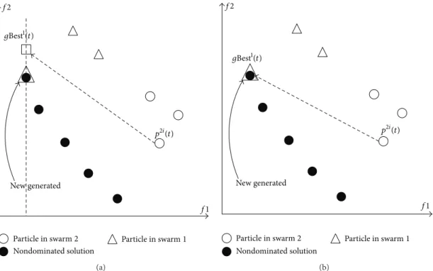
Thus, the use of nondominated solutions to enhance the VEPSO algorithm can be further improved by the use of multileader concept in this work. According to (6), which is the velocity equation of the VEPSO, the particles of a swarm are guided by its 𝑝Best(𝑡) and another swarm’s 𝑔Best(𝑡). For example, as shown inFigure 4(a), the particles from the second swarm optimise the second objective function using
𝑔Best1(𝑡)only, which may not be the solution that has the best fitness with respect to the second objective function. Thus, this original mechanism of VEPSO may limit the convergence rate of the algorithm. Therefore, an improved VEPSO algorithm is proposed by including 𝑔Best2(𝑡) as additional guidance to optimise both objective functions, as shown inFigure 4(b).
Hence, the general velocity equation of this improved VEPSO is formulated as in (9) V𝑚𝑛𝑖 (𝑡 + 1) = 𝜒 [𝜔V𝑚𝑖𝑛 (𝑡) + 𝑐1𝑟1(𝑝Best𝑚𝑖𝑛 − 𝑝𝑚𝑖𝑛 (𝑡)) +∑𝑀 𝑞=1𝑐 𝑞 2𝑟2𝑞(𝑔Best𝑞𝑛− 𝑝𝑚𝑖𝑛 (𝑡))] , (9)
where for each 𝑞, 𝑐2𝑞, and 𝑟2𝑞 are independent constant and random values, respectively. In addition, from (9), as compared to the improved VEPSO at previous section, the particles will search toward the nondominated solutions which located at different end of the Pareto front. Therefore,
f2
f1 New generated
p2i(t)
Particle in swarm2 Particle in swarm1
gBest1(t) Nondominated solution (a) f2 f1 New generated p2i(t)
Particle in swarm2 Particle in swarm1
gBest1(t)
Nondominated solution (b)
Figure 3: (a) Particles guided by the best solution from the other swarm (b) Particles guided by a nondominated solution with respect to another swarm.
f2
f1 New generated
p2i(t)
Particle in swarm2 Particle in swarm1
gBest1(t) Nondominated solution (a) f2 f1 New generated
Particle in swarm2 Particle in swarm1
p2i(t)
gBest1(t)
gBest2(t)
Nondominated solution (b)
Figure 4: (a) A particle is guided based on𝑔Best1(𝑡). (b) A particle is guided based on𝑔Best1(𝑡)and𝑔Best2(𝑡).
the diversity performance of the algorithm is expected to be better as the search area is wider, rather than a single point.
Because the improved VEPSO algorithm uses multiple nondominated solutions as particle guides, or leaders, this algorithm is called VEPSO using multiple nondominated leaders (VEPSOml). Also, a polynomial mutation mecha-nism from NSGA-II [14] is used to modify particle positions
at some probability. By mutating the position of some particles out of the locally optimal solution, this mechanism broadens the search for a globally optimal solution. In this study, the position of one out of every fifteen particles is mutated in the algorithm. Therefore, the complete VEPSO algorithm using multiple nondominated leaders is shown in
begin
Initialiseposition&velocityfor allM-swarm; Evaluateobjectivefor allM-swarm;
Initialisearchive;
InitialisepBest for allM-swarm; InitialisegBest (8) for allM-swarm;
while𝑖 ≤ 𝑖maxdo
Updatevelocity(9) for allM-swarm; Updateposition(4) for allM-swarm; Mutatepositionfor allM-swarm; Evaluateobjectivefor allM-swarm; Updatearchive;
UpdatepBest for allM-swarm; UpdategBest (8) for allM-swarm;
𝑖++;
end end
Algorithm 3: The VEPSO algorithm using multinondominated leaders.
4. Experiment
4.1. Performance Measure. MOO algorithms face difficulty in converging to and distributing the nondominated solutions over the true Pareto front,PF𝑡. Hence, the algorithm per-formance is measured by the quality of the obtained Pareto front, PF𝑜. Several performance measures are used for comparison to highlight any improvement in the proposed algorithm.
The number of solutions (NS) measured will calculate the total number of nondominated solutions found by an algorithm. The best algorithm, by this measure, gives the most nondominated solutions. A more advanced measure uses the generalized distance (GD) [18], which is a popular measure of convergence [14]. This performance measure first evaluates the average distance between the true Pareto front and the one obtained by the algorithm. Equation (10) is used to compute the average distance, with a smaller value corresponding to a better performance. Then, the minimum distance of a nondominated solution from the true Pareto front is calculated using (11)
GD= (∑ ‖PF𝑜‖ 𝑞=1 𝑑𝑀𝑞 ) 1/𝑀 PF𝑜 (10) 𝑑𝑞= min 1≤𝑔≤‖PF𝑡‖√ 𝑀 ∑ 𝑚=1 (PF𝑚 𝑜 𝑞−PF𝑚𝑡 𝑔)2. (11)
In addition, SP [14] is a commonly used measure of the diversity performance, or the distribution of nondominated solutions [14] is used. Equations (12), (13), and (14) evaluate the diversity performance, as measured by SP. The𝑑𝑓and𝑑𝑙 are the Euclidean distances between the boundary solution and the nondominated solutions returned by the algorithm and the true Pareto front, respectively. The Euclidean distance between two solutions can be calculated using (13). Thus, SP actually measures the average distance of one solution and of the next solution to all nondominated solutions returned
by the algorithm as well as two boundary solutions in the true Pareto front. Hence, it is desirable that the Pareto front returned by the algorithm produces a small SP:
Spread=𝑑𝑓+ 𝑑𝑙+ ∑ ‖PF𝑜‖−1 𝑞=1 𝑑𝑞− 𝑑 𝑑𝑓+ 𝑑𝑙+ 𝑑 (PF𝑜 − 1) , (12) 𝑑𝑞= √(PF1 𝑜𝑞−PF1𝑜𝑞+1) 2 + (PF2 𝑜𝑞−PF2𝑜𝑞+1) 2 , (13) 𝑑 = ∑ ‖PF𝑜‖−1 𝑞=1 𝑑𝑞 PF𝑜 − 1 . (14)
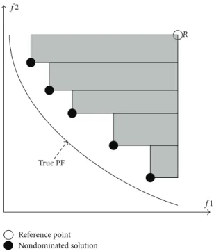
Additionally, the hypervolume (HV) [19] measures the area (in a two-objective problem) or the volume between a reference point, 𝑅 and the Pareto front with respect to the nondominated solutions obtained by the algorithm, as illustrated in Figure 5. Thus, it is desirable that the Pareto front returned by the algorithm produces a large HV.
4.2. Test Problems. Because different features in MOO prob-lems are responsible for decreasing the likelihood of obtain-ing Pareto front with good convergence and diversity, the standard test functions with well-defined true Pareto fronts are important for testing optimisation algorithms. Five test functions from Zitzler et al. [20] (ZDT) are used here for this reason. The ZDT test problems have two objectives and are formulated with one feature in each problem. ZDT5 is not used because it is binary coded, whereas this work focuses on real-value problems. During testing, the GD, SP, and HV measure require the true Pareto front for the ZDT test problems, the standard database generated by jMetal (http://jmetal.sourceforge.net/problems.html) is used for this purpose. Additionally, all test problems used here are set up as recommended by [20].
4.3. Evaluation of VEPSO Algorithms. The performance comparison between conventional VEPSO, VEPSOnds, and
f2 f1 Reference point R TruePF Nondominated solution
Figure 5: Hypervolume measure with area covered by nondominated solutions and reference point.
Table 1: Algorithm parameters.
Parameter Value
Function evaluation 25000 (based on paper [14])
(i) Number of swarm 2
(ii) Particle for each swarm 50 (iii) Iterations for each run 250
𝑐1and𝑐2 Random [1.5, 2.5]
𝜔 Linearly degrade from 1.0 to 0.4
VEPSOml is conducted without the use of polynomial mutation as to clarify that the polynomial mutation is not the sole reason for any performance improvement. Thus, this experiment compares the conventional VEPSO and the VEPSOnds without mutation against two different variations of VEPSOml: VEPSOml1 is the VEPSOml without mutation and VEPSOml2 is the VEPSOml with mutation, respectively. All improved VEPSO algorithms are compared to the conventional VEPSO algorithm. Hence, similar parameters are used for all experimented algorithms which are listed in
Table 1. In addition, the archive size is set to 100 solutions and is controlled by removing the nondominated solutions with the smallest crowding distance [14]. Each test problem is simulated for 100 runs on each algorithm to obtain statistical results for a fair comparison because the convergence and diversity performance varies in each run.
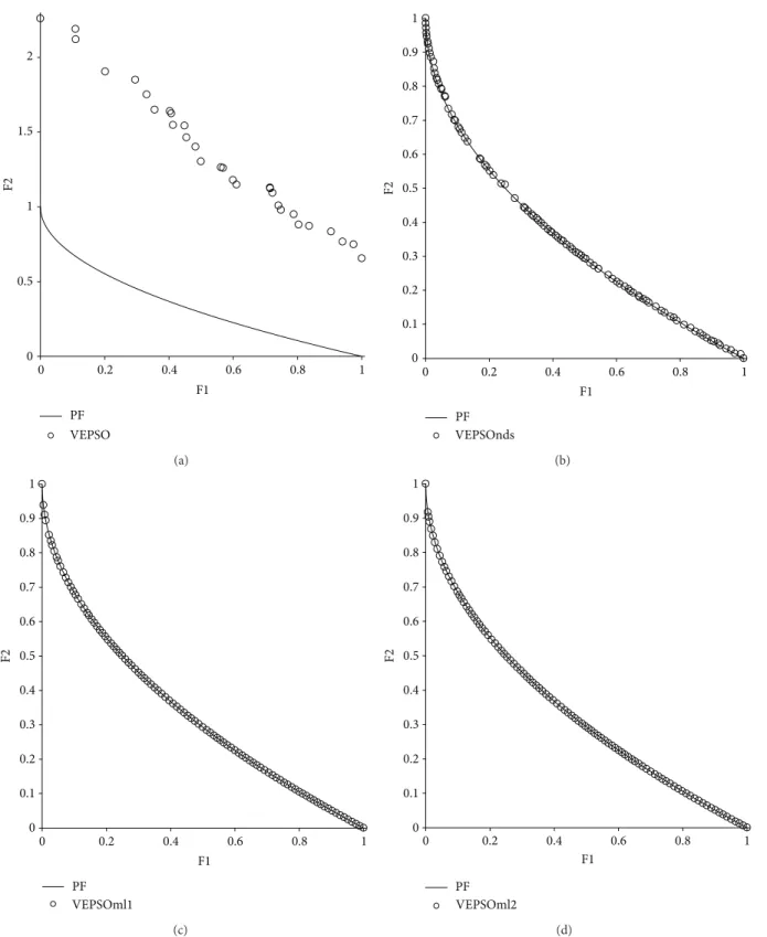
Table 2 lists the performance of each algorithm on the ZDT1 test problem. In the NS measure, the number of non-dominated solutions significantly increases in all improved algorithms. Under the GD measure, VEPSOnds performs approximately 10 times better than conventional VEPSO. However, under the same measure, VEPSOml1 shows a more
dramatic improvement, performing approximately 100 times better than VEPSO, as the concept of multiple nondominated leaders shows its benefit in finding more accurate solutions. Additionally, when the polynomial mutation is included, as in VEPSOml2, the GD performance improved much better at about 600% as compared to the conventional VEPSO. Under the SP measure, VEPSOnds also gives a significant improvement in performance. Meanwhile, the VEPSOml1 and VEPSOml2 show significant improvement in diversity performance as compared to the VEPSOnds. This shows the significance of using more than one nondominated solution which diversify the search toward the nondominated solu-tions at different end. The above mentioned improvements are supported by the higher HV measures when compared to the conventional VEPSO, which indicates that they return better Pareto fronts.
Figure 6shows plots of the nondominated solutions with the best GD measure returned by each algorithm tested on ZDT1. From the first plot, it is clear that the nondominated solutions obtained by VEPSO are far away from the true Pareto front, which explains the poor performance of this algorithm for this test problem. In addition, the nondomi-nated solutions are distributed unevenly, and so VEPSO has a larger SP value. Meanwhile for all the improved VEPSO algorithms, their nondominated solutions fall very close to the true Pareto front. However, VEPSOnds produces a distribution of nondominated solutions that contain empty spaces along the true Pareto front, which results in higher SP value as compared to the other improved VEPSO algorithms.
Table 3 lists the performance of the algorithms on the ZDT2 test problem. The average number of nondominated solutions found by VEPSOnds1 slightly improves over the number found by VEPSO, but VEPSOnds2, VEPSOml1, and VEPSOml2 greatly improve over VEPSO by this same
0 2 1.5 1 0.5 0 0.2 0.4 0.6 0.8 1 F 2 F1 PF VEPSO (a) 1 PF 0.9 0.8 0.7 0.6 0.5 0.4 0.3 0.2 0.1 0 VEPSOnds 0 0.2 0.4 0.6 0.8 1 F 2 F1 (b) VEPSOml1 1 PF 0.9 0.8 0.7 0.6 0.5 0.4 0.3 0.2 0.1 0 0 0.2 0.4 0.6 0.8 1 F 2 F1 (c) VEPSOml2 1 PF 0.9 0.8 0.7 0.6 0.5 0.4 0.3 0.2 0.1 0 0 0.2 0.4 0.6 0.8 1 F 2 F1 (d)
Figure 6: Plot of nondominated solutions returned by each algorithm for the ZDT1 test problem.
measure. Similarly, by the GD measure, VEPSOnds1 shows a small improvement, whereas VEPSOnds2 and VEPSOml1 show a larger improvement over the performance of VEPSO. In the same measure, VEPSOml2 shows a more significant improvement over the VEPSO and all other improved algo-rithms. Additionally, by the SP measure, VEPSOnds1 shows
negligible improvement, whereas VEPSOnds2 shows a signif-icant improvement over the performance of VEPSO. Besides, with the use of multileader, VEPSOml shows much better diversity performance than both the VEPSOnds. Finally, by the HV measure, VEPSO was unable to produce any hypervolume because its nondominated solutions are worse
0 2.5 2 1.5 1 0.5 0 0.2 0.4 0.6 0.8 1 F 2 F1 PF VEPSO (a) 1 0.9 0.8 0.7 0.6 0.5 0.4 0.3 0.2 0.1 0 0 0.2 0.4 0.6 0.8 1 F 2 F1 PF VEPSOnds (b) VEPSOml1 1 0.9 0.8 0.7 0.6 0.5 0.4 0.3 0.2 0.1 0 0 0.2 0.4 0.6 0.8 1 F 2 F1 PF (c) VEPSOml2 1 0.9 0.8 0.7 0.6 0.5 0.4 0.3 0.2 0.1 0 0 0.2 0.4 0.6 0.8 1 F 2 F1 PF (d)
Figure 7: Plot of nondominated solutions returned by each algorithm for the ZDT2 test problem.
than the reference point,𝑅. On the other hand, all improved algorithms are able to create a hypervolume, especially the VEPSOml2 which produce the largest hypervolume.
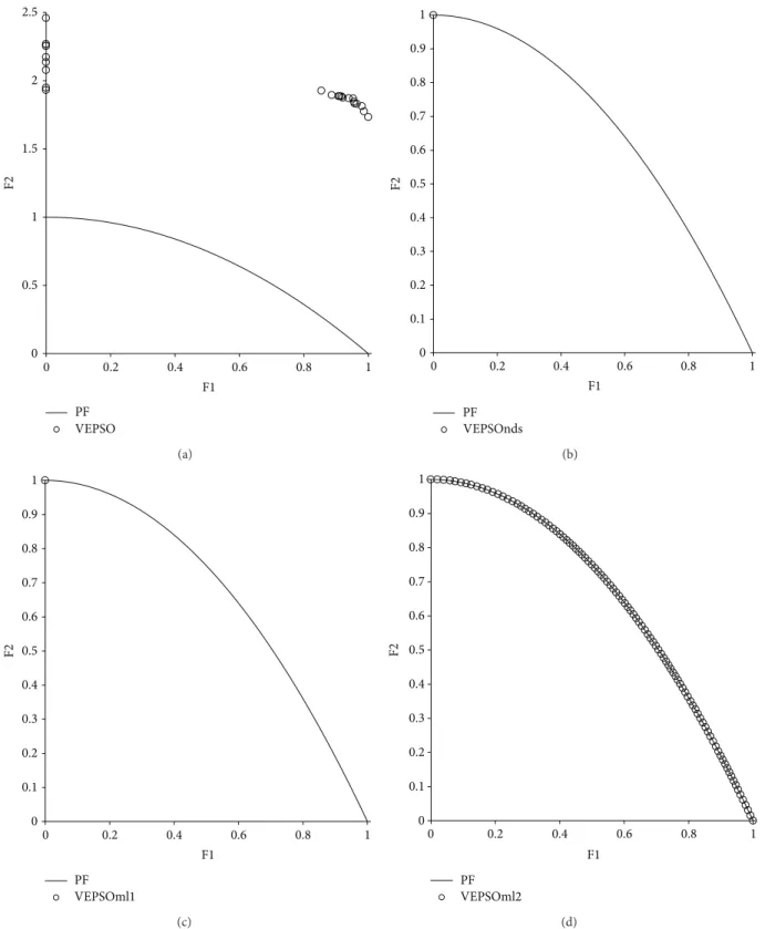
Figure 7displays the nondominated solutions, plotted for each the best GD measure obtained for each algorithm using
the ZDT2 test problem. The first plot shows that VEPSO returns nondominated solutions that are far from the true Pareto font and poorly distributed. Although VEPSOnds and VEPSOml1 return a low GD measure, the number of nondominated solutions is found to have low value, which
3.2 2.7 2.2 1.7 1.2 1 −0.8 0.8 0.7 0.6 0.4 −0.3 0.2 0.2 0 F 2 F1 PF VEPSO (a) 1 −0.8 0.8 −0.6 0.6 −0.4 0.4 −0.2 0.2 0 0 0.2 0.4 0.6 0.8 1 F 2 F1 PF VEPSOnds (b) VEPSOml 1 −0.8 0.8 −0.6 0.6 −0.4 0.4 −0.2 0.2 0 0 0.2 0.4 0.6 0.8 1 F 2 F1 PF (c) VEPSOm2 1 −0.8 0.8 −0.6 0.6 −0.4 0.4 −0.2 0.2 0 0 0.2 0.4 0.6 0.8 1 F 2 F1 PF (d)
Figure 8: Plot of nondominated solutions returned by each algorithm for the ZDT3 test problem.
is clearly displayed in the second and third plots, respectively, ofFigure 6. In fact, there is only one nondominated solution found by both algorithms which falls exactly on the true Pareto front and yields a GD value of zero. On the other hand, the fourth plot of Figure 6 shows that VEPSOml2 returns the nondominated solutions that converge nicely and are well distributed over the true Pareto front. Besides, the nondominated solutions found by VEPSOml2 distributed evenly which yield a good SP value.
Table 4 lists the performance of the algorithms on the ZDT3 test problem. All improved VEPSO algorithms are able to find more nondominated solutions than the conventional VEPSO algorithm. In addition, the performances of the improved VEPSO algorithms, with respect to convergence, improve on conventional VEPSO, while VEPSOml2 shows the greater improvement. However, by the SP measure, the VEPSOnds algorithm performs worse than the conventional VEPSO algorithm. However, although the SP value of the
Table 2: Algorithm performance tested on ZDT1 problem.
Measure VEPSO VEPSOnds VEPSOml1 VEPSOml2
NS Ave. 30.220000 100.000000 99.490000 98.820000 SD 5.697031 0.000000 3.942760 6.979595 Min. 16.000000 100.000000 63.000000 47.000000 Max. 44.000000 100.000000 100.000000 100.000000 GD Ave. 0.295865 0.022637 0.002730 0.000497 SD 0.051645 0.014201 0.006219 0.002213 Min. 0.139491 0.000283 0.000045 0.000047 Max. 0.432478 0.073477 0.031891 0.015598 SP Ave. 0.834481 0.729350 0.212479 0.182157 SD 0.039111 0.160298 0.149696 0.113453 Min. 0.705367 0.322322 0.106082 0.109998 Max. 0.917087 1.219625 0.738619 0.779572 HV Ave. 0.001886 0.428153 0.628841 0.657830 SD 0.010058 0.113432 0.078273 0.023359 Min. — 0.185313 0.283932 0.456556 Max. 0.087426 0.659603 0.662065 0.662022
Table 3: Algorithm performance tested on ZDT2 problem.
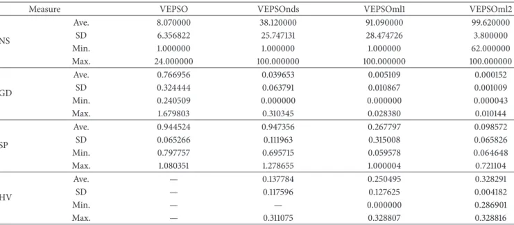
Measure VEPSO VEPSOnds VEPSOml1 VEPSOml2
NS Ave. 8.070000 38.120000 91.090000 99.620000 SD 6.356822 25.747131 28.474726 3.800000 Min. 1.000000 1.000000 1.000000 62.000000 Max. 24.000000 100.000000 100.000000 100.000000 GD Ave. 0.766956 0.039653 0.005109 0.000152 SD 0.324444 0.063791 0.010867 0.001009 Min. 0.240509 0.000000 0.000000 0.000043 Max. 1.679803 0.310345 0.028380 0.010144 SP Ave. 0.944524 0.947356 0.267797 0.098572 SD 0.065266 0.111963 0.315008 0.065826 Min. 0.797757 0.695715 0.059578 0.064648 Max. 1.080351 1.278655 1.000004 0.721104 HV Ave. — 0.137784 0.250495 0.328291 SD — 0.117596 0.127625 0.004182 Min. — — 0.000000 0.286901 Max. — 0.311075 0.328807 0.328816
conventional VEPSO algorithm is better, the superior conver-gence of the VEPSOnds algorithm maintains its performance advantage. In contrast, both improved VEPSO algorithm using multiple nondominated leaders show better SP mea-sure than the conventional VEPSO, which strengthen the hypothesis that using multiple nondominated leaders will improve diversity performance. In addition, the HV value of the conventional VEPSO algorithm is smaller than of all improved algorithms which suggest that the improved algorithms have better performance.
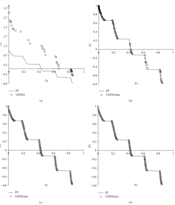
Figure 8displays the nondominated solutions, plotted for the best GD measure obtained for each algorithm using the ZDT3 test problem. The nondominated solutions returned by the conventional VEPSO algorithm were distributed equally but not well converged with respect to the true Pareto front.
On the other hand, the nondominated solutions from all improved VEPSO algorithms are well converged with respect to the true Pareto front. However, the nondominated solu-tions returned by the VEPSOnds algorithm are denser at the upper left of the Pareto front, which causes the increase in its SP value. In contrast, the nondominated solutions obtained by both VEPSOml algorithms are equally distributed over the Pareto front and yield better SP value.
Table 5 lists the performance of the algorithms on the ZDT4 test problem. The average number of nondominated solutions obtained by VEPSO is relatively low, while all improved VEPSO algorithms found most of the solutions. In this test, the conventional VEPSO algorithm produced a very large GD value due to the multimodality feature in the test problem, and so the improved VEPSO algorithms
Table 4: Algorithm performance tested on ZDT3 problem.
Measure VEPSO VEPSOnds VEPSOml1 VEPSOml2
NS Ave. 35.150000 99.600000 95.710000 96.500000 SD 6.853997 3.405284 11.528003 11.372037 Min. 21.000000 66.000000 46.000000 49.000000 Max. 53.000000 100.000000 100.000000 100.000000 GD Ave. 0.173060 0.009607 0.002586 0.001456 SD 0.031253 0.008293 0.003904 0.002533 Min. 0.079595 0.000433 0.000153 0.000159 Max. 0.276801 0.039481 0.017547 0.007328 SP Ave. 0.871146 1.109448 0.761061 0.752151 SD 0.043319 0.086041 0.056129 0.050459 Min. 0.701884 0.902861 0.701924 0.703181 Max. 1.001428 1.322024 0.934796 0.981492 HV Ave. 0.004722 0.373133 0.476679 0.493073 SD 0.021699 0.083015 0.060626 0.045211 Min. — 0.112859 0.289513 0.391275 Max. 0.167359 0.506222 0.515919 0.515941
Table 5: Algorithm performance tested on ZDT4 problem.
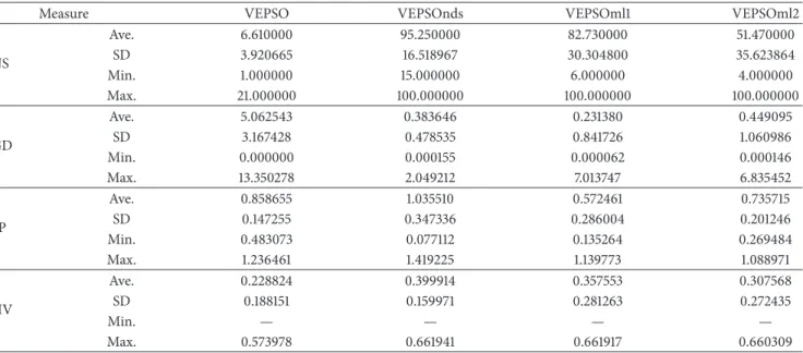
Measure VEPSO VEPSOnds VEPSOml1 VEPSOml2
NS Ave. 6.610000 95.250000 82.730000 51.470000 SD 3.920665 16.518967 30.304800 35.623864 Min. 1.000000 15.000000 6.000000 4.000000 Max. 21.000000 100.000000 100.000000 100.000000 GD Ave. 5.062543 0.383646 0.231380 0.449095 SD 3.167428 0.478535 0.841726 1.060986 Min. 0.000000 0.000155 0.000062 0.000146 Max. 13.350278 2.049212 7.013747 6.835452 SP Ave. 0.858655 1.035510 0.572461 0.735715 SD 0.147255 0.347336 0.286004 0.201246 Min. 0.483073 0.077112 0.135264 0.269484 Max. 1.236461 1.419225 1.139773 1.088971 HV Ave. 0.228824 0.399914 0.357553 0.307568 SD 0.188151 0.159971 0.281263 0.272435 Min. — — — — Max. 0.573978 0.661941 0.661917 0.660309
clearly performed better in this respect. However, the diver-sity performance of nondominated solutions returned by conventional VEPSO is small compared to the VEPSOnds algorithm. Once again, the use of multiple nondominated leaders in VEPSO algorithms could diversify the search and result in better diversity performance. Additionally, all algorithms produce a hypervolume from the reference point, and all improved algorithms return larger HV values than the conventional algorithm.
Figure 9 displays the nondominated solutions, plotted for the best GD measure obtained for each algorithm using the ZDT4 test problem. The first plot shows that VEPSO converges to the Pareto front but only manages to obtain a single nondominated solution. The VEPSOnds algorithm not
only converges to the Pareto front but also returns a diverse set of nondominated solutions. On the other hands, both VEPSOml also returned the nondominated solutions with good convergence but they are not well distributed as com-pared to the VEPSOnds, in this case. Thus, the VEPSOnds shows better HV value as compared to the VEPSOml.
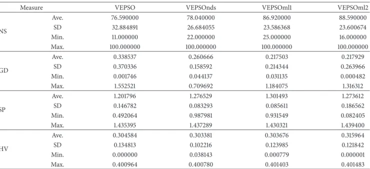
Table 6 lists the performance of the algorithms on the ZDT6 test problem. All algorithms find a similar number of nondominated solutions. In the GD measure, all algorithms are capable of returning the nondominated solutions that converge well to the Pareto front. On the other hand, both VEPSOml1 and VEPSOml2 algorithms outperform the conventional VEPSO and VEPSOnds algorithm in the GD measure. In addition, the SP and HV values for each
Table 6: Algorithm performance tested on ZDT6 problem.
Measure VEPSO VEPSOnds VEPSOml1 VEPSOml2
NS Ave. 76.590000 78.040000 86.920000 88.590000 SD 32.884891 26.684055 23.586368 23.600674 Min. 11.000000 22.000000 25.000000 16.000000 Max. 100.000000 100.000000 100.000000 100.000000 GD Ave. 0.338537 0.260666 0.217503 0.217929 SD 0.370336 0.158592 0.214344 0.263966 Min. 0.001746 0.044137 0.031135 0.000482 Max. 1.552521 0.709692 1.184075 1.316312 SP Ave. 1.201796 1.276529 1.301493 1.273612 SD 0.146782 0.083293 0.085611 0.186562 Min. 0.492064 0.987981 0.931549 0.082405 Max. 1.435395 1.437289 1.430321 1.439400 HV Ave. 0.304584 0.303381 0.303676 0.315964 SD 0.134813 0.102216 0.123985 0.121842 Min. 0.000000 0.038143 0.000779 0.000001 Max. 0.400964 0.400780 0.401403 0.401483
algorithm are similar. However, the VEPSOml2 algorithm shows superiority in getting the minimum SP value and average HV value.
As can be predicted from the similar quantitative per-formance of the algorithms on ZDT6, the plot of non-dominated solutions returned by each algorithm is very similar, especially in convergence performance, as shown in
Figure 10. The plots do show that VEPSO has slightly less diversity compared to VEPSOnds and VEPSOml2 because of some small gaps in coverage along the middle of the Pareto front. On the other hand, the VEPSOml1 shows weak distribution of nondominated solutions over the Pareto front. In contrast, the nondominated solutions found by VEPSOnds and VEPSOml2 completely cover the true Pareto front and are spaced out equally.
As seen from the results of all the test problems, the VEPSO algorithms using multiple nondominated leaders shows more improvement in terms of convergence and diversity of the nondominated solutions found than the VEP-SOnds. The additional leader, specifically the nondominated solution with respect to the objective function optimised by a swarm, not only guides the particles to optimise the objective function with respect to the swarm. It also increased the search area because all leaders used to guide the particles are located at the different end of the Pareto front.
4.4. Analysis of the Number of Particles. This experiment analysed the performance of the VEPSOml2 algorithm with various numbers of particles. Similar parameters from the previous experiment were used except for the total number of particles as it is equally divided into two swarms; the total number of particles was varied to be 10, 30, 50, 100, 300, 500, and 1000.Figure 11shows plots of the performance measures for each benchmark problem against the total number of particles.
The VEPSOml2 algorithm performance improved as the number of particles increased. The performance of the VEPSOml2 algorithm was sufficient when there were 100 particles computed for 250 iterations, which corresponds to 25000 function evaluations. However, the performance of the VEPSOml2 algorithm exhibited better results when the total number of particles was increased. Unfortunately, when the number of particles is increased, the algorithm requires more computational effort to solve the problem.
4.5. Analysis of the Number of Iterations. This experiment investigated the performance of VEPSOml2 for various numbers of iterations. The number of iterations was fixed to be 10, 30, 50, 100, 300, 500, 1000, 3000, 5000, and 10 000. Meanwhile, the other parameters were kept the same as in the previous experiment except that the number of particles, which were divided equally among swarms, was fixed to 100 divided equally between all swarms.Figure 12plots the performance measures for each benchmark problem against the number of iterations.
As expected, the performance of VEPSOml2 is improved when the number of iterations was increased. When 100 particles were used, the VEPSOml2 algorithm started to yield acceptable results when there were 500 iterations, which is equivalent to 50000 function evaluations. However, if computational cost is not critical, the VEPSOml2 algorithm could use 3000 iterations because the performance saturated after this value.
4.6. Benchmarking with the State-of-the-Art Multiobjec-tive Optimisation Algorithms. For benchmarking, the VEP-SOml2 algorithm was compared to four other state-of-the-art MOO algorithms: nondominated sorting genetic algorithm-II (NSGA-II) [14], strength Pareto evolutionary algorithm2(SPEA2) [21], archive-based hybrid scatter search
1 0.9 0.8 0.7 0.6 0.5 0.4 0.3 0.2 0.1 0 0 0.2 0.4 0.6 0.8 1 F 2 F1 PF VEPSO (a) VEPSOnds 1 0.9 0.8 0.7 0.6 0.5 0.4 0.3 0.2 0.1 0 0 0.2 0.4 0.6 0.8 1 F 2 F1 PF (b) 1 VEPSOml1 1 0.9 0.8 0.7 0.6 0.5 0.4 0.3 0.2 0.1 0 0 0.2 0.4 0.6 0.8 1 F 2 F1 PF (c) VEPSOml2 1 0.9 0.8 0.7 0.6 0.5 0.4 0.3 0.2 0.1 0 0 0.2 0.4 0.6 0.8 1 F 2 F1 PF (d)
Figure 9: Plot of nondominated solutions returned by each algorithm for the ZDT4 test problem.
(AbYSS) [22], and the speed-constrained multiobjective PSO (SMPSO) algorithm [23]. All algorithms only computed 25000 function evaluations, and the archive size was set to 100 for fair comparison. The population size for NSGA-II was set to 100 for optimisation. The Simulated Binary Crossover
(SBX) operator was used with crossover probability𝑝𝑐= 0.9. The polynomial mutation [24] operator was also used with mutation probability𝑝𝑚 = 1/𝑁. Meanwhile, the distribution indices for both operators were set to𝜇𝑛 = 𝜇𝑚 = 20. The parameters in SPEA2 were set the same as in NSGA-II. The
1 0.8 0.6 0.4 0.2 0 0.2 0.4 0.6 0.8 1 F1 PF VEPSO F 2 (a) 1 0.9 0.8 0.7 0.6 0.5 0.4 0.3 0.2 0.1 0 0.2 0.4 0.6 0.8 1 F 2 F1 PF VEPSOnds (b) 1 0.9 0.8 0.7 0.6 0.5 0.4 0.3 0.2 0.1 0 0.2 0.4 0.6 0.8 1 F 2 F1 PF VEPSOml1 (c) 0.2 0.4 0.6 0.8 1 F 2 F1 PF VEPSOml2 1 0.9 0.8 0.7 0.6 0.5 0.4 0.3 0.2 0.1 0 (d)
120 100 80 60 40 20 0 10 100 1000 NS ZDT1 ZDT2 ZDT3 ZDT4 ZDT6 (a) 1 0.9 0.8 0.7 0.6 0.5 0.4 0.3 0.2 0.1 0 10 100 1000 GD ZDT1 ZDT2 ZDT3 ZDT4 ZDT6 (b) 1.4 1.2 1 0.8 0.6 0.4 0.2 0 10 100 1000 Spread ZDT1 ZDT2 ZDT3 ZDT4 ZDT6 (c) 0.7 0.6 0.5 0.4 0.3 0.2 0.1 0 10 100 1000 HV ZDT1 ZDT2 ZDT3 ZDT4 ZDT6 (d)
Figure 11: Plots of the performance measures versus numbers of particles. (a) Number of solutions. (b) Generational distance. (c) Spread. (d) Hypervolume.
population size for AbYSS was set to 20 and the pairwise combination parameters𝑅𝑒𝑓𝑆𝑒𝑡1and𝑅𝑒𝑓𝑆𝑒𝑡2were both set to 10. In addition, the polynomial mutation parameters in AbYSS were also set similarly as in NSGA-II and SPEA2. Finally, SMPSO was set to have a population size of 100 particles and a total number of iterations of 250. Moreover, the𝑟1 = 𝑟2 = random[0.1, 0.5], and the terms𝑐1 = 𝑐2 =
random[1.5, 2.0]. The polynomial mutation [25] operator was also used in SMPSO with𝑝𝑚= 1/𝑁and𝜇𝑚= 20.
The performance measures for the ZDT1 problem for all algorithms are listed inTable 7. The average number of solutions obtained by the VEPSOml2 was very similar to the other algorithms. Although VEPSOml2 algorithm had a GD measure approximately twice as large as those of the other
120 100 80 60 40 20 0 10 100 1000 10000 NS ZDT1 ZDT2 ZDT3 ZDT4 ZDT6 (a) GD 1.4 1.6 1.2 1 0.8 0.6 0.4 0.2 0 10 100 1000 10000 ZDT1 ZDT2 ZDT3 ZDT4 ZDT6 (b) 1.4 1.2 1 0.8 0.6 0.4 0.2 0 10 100 1000 10000 Spread ZDT1 ZDT2 ZDT3 ZDT4 ZDT6 (c) 0 0.1 0.2 0.3 0.4 0.5 0.6 0.7 10 100 1000 10000 HV ZDT1 ZDT2 ZDT3 ZDT4 ZDT6 (d)
Figure 12: Plots of the performance metrics for various numbers of iterations. (a) Number of solution. (b) Generational distance. (c) Spread. (d) Hypervolume.
algorithms, its minimum GD was still the smallest among them. However, the SP was, on average, better than NSGA-II. Interestingly, the HV measure of VEPSOml2 was as good as those of the other algorithms.
Table 8 presents the performance measure of the algo-rithms for the ZDT2 problem. The VEPSOml2 was suf-ficiently competitive at obtaining a reasonable number of solutions. In the GD measure, on average, the VEPSOml2
Table 7: Performance comparison based on ZDT1 test problem.
Measure AbYSS NSGA-II SPEA2 SMPSO VEPSOml2
NS Ave. 100.000000 100.000000 100.000000 100.000000 98.820000 SD 0.000000 0.000000 0.000000 0.000000 6.979595 Min. 100.000000 100.000000 100.000000 100.000000 47.000000 Max. 100.000000 100.000000 100.000000 100.000000 100.000000 GD Ave. 0.000185 0.000223 0.000220 0.000117 0.000497 SD 0.000035 0.000038 0.000028 0.000031 0.002213 Min. 0.000125 0.000146 0.000154 0.000053 0.000047 Max. 0.000343 0.000374 0.000400 0.000172 0.015598 SP Ave. 0.105387 0.379129 0.148572 0.076608 0.182157 SD 0.012509 0.028973 0.012461 0.009200 0.113453 Min. 0.080690 0.282485 0.116765 0.056009 0.109998 Max. 0.136747 0.441002 0.174986 0.099653 0.779572 HV Ave. 0.661366 0.659333 0.659999 0.661801 0.657830 SD 0.000269 0.000301 0.000301 0.000100 0.023359 Min. 0.660267 0.658486 0.659347 0.661372 0.456556 Max. 0.661724 0.659909 0.660629 0.661991 0.662022
Table 8: Performance comparison based on ZDT2 test problem.
Measure AbYSS NSGA-II SPEA2 SMPSO VEPSOml2
NS Ave. 100.000000 100.000000 100.000000 100.000000 99.620000 SD 0.000000 0.000000 0.000000 0.000000 3.800000 Min. 100.000000 100.000000 100.000000 100.000000 62.000000 Max. 100.000000 100.000000 100.000000 100.000000 100.000000 GD Ave. 0.000131 0.000176 0.000182 0.000051 0.000152 SD 0.000067 0.000066 0.000039 0.000003 0.000152 Min. 0.000056 0.000093 0.000090 0.000044 0.000043 Max. 0.000433 0.000707 0.000304 0.000060 0.010144 SP Ave. 0.130425 0.378029 0.158187 0.071698 0.098572 SD 0.090712 0.028949 0.027529 0.013981 0.065826 Min. 0.080831 0.311225 0.118114 0.035786 0.064648 Max. 0.833933 0.430516 0.365650 0.106749 0.721104 HV Ave. 0.325483 0.326117 0.326252 0.328576 0.328291 SD 0.023209 0.000297 0.000908 0.000077 0.004182 Min. 0.096409 0.325278 0.318785 0.328349 0.286901 Max. 0.328505 0.326696 0.327559 0.328736 0.328816
algorithm was as good as the other algorithms, but SMPSO had greater performance. Surprisingly, the VEPSOml2 algo-rithm was able to obtain a better minimum GD measure than the SMPSO algorithm. Additionally, the SP measure of the VEPSOml2 algorithm was better than those of the other algorithms except SMPSO. All algorithms had similar HV values, but VEPSOml2 yielded the best HV performance.
The performance measures for the ZDT3 problem for all algorithms are listed inTable 9. Both SMPSO and VEPSOml2 were unable to obtain the maximum number of solutions consistently for all 100 runs but still yielded solutions within a reasonable range. Noticeably, the average GD measure for VEPSOml2 was the largest among all algorithms. However,
the diversity for VEPSOml2 was similar to that of the others. Moreover, although the HV value of VEPSOml2 was the smallest, it still yielded a very large HV.
Table 10 presents the performance measures for the algorithms for the ZDT4 problem. VEPSOml2 faced great challenges from the multiple local optima featured in this problem, where it cause the algorithm to obtain a very small number of solutions. Additionally, the convergence and diversity of VEPSOml2 were bad, as indicated by the very large GD and SP values. As expected, the HV performance was also very poor because the multiple local optima feature is one of the natural weaknesses of PSO-based algorithms [26,27].
Table 9: Performance comparison based on ZDT3 test problem.
Measure AbYSS NSGA-II SPEA2 SMPSO VEPSOml2
NS Ave. 100.000000 100.000000 100.000000 99.900000 96.500000 SD 0.000000 0.000000 0.000000 0.904534 11.372037 Min. 100.000000 100.000000 100.000000 91.000000 49.000000 Max. 100.000000 100.000000 100.000000 100.00000 100.000000 GD Ave. 0.000193 0.000211 0.000230 0.000203 0.001456 SD 0.000019 0.000013 0.000019 0.000061 0.002533 Min. 0.000144 0.000180 0.000184 0.000155 0.000159 Max. 0.000264 0.000268 0.000327 0.000717 0.007328 SP Ave. 0.707651 0.747853 0.711165 0.717493 0.752151 SD 0.013739 0.015736 0.008840 0.032822 0.050459 Min. 0.696859 0.715199 0.698590 0.697943 0.703181 Max. 0.796404 0.793183 0.775317 0.950901 0.981492 HV Ave. 0.512386 0.514813 0.513996 0.514996 0.493073 SD 0.011314 0.000159 0.000675 0.001737 0.045211 Min. 0.463776 0.514449 0.510764 0.500484 0.391275 Max. 0.515960 0.515185 0.514668 0.515818 0.515941
Table 10: Performance comparison based on ZDT4 test problem.
Measure AbYSS NSGA-II SPEA2 SMPSO VEPSOml2
NS Ave. 99.680000 100.000000 100.000000 100.000000 51.470000 SD 3.100603 0.000000 0.000000 0.000000 35.623864 Min. 69.000000 100.000000 100.000000 100.000000 4.000000 Max. 100.000000 100.000000 100.000000 100.000000 100.000000 GD Ave. 0.001231 0.000486 0.000923 0.0001347 0.449095 SD 0.002632 0.000235 0.001428 0.000027 1.060986 Min. 0.000148 0.000163 0.000176 0.000070 0.000146 Max. 0.014472 0.001374 0.012292 0.000187 6.835452 SP Ave. 0.159842 0.392885 0.298269 0.092281 0.735715 SD 0.120180 0.037083 0.125809 0.011777 0.201246 Min. 0.078244 0.324860 0.137934 0.067379 0.269484 Max. 1.073669 0.473358 0.884091 0.124253 1.088971 HV Ave. 0.646058 0.654655 0.645336 0.661401 0.307568 SD 0.034449 0.003406 0.018773 0.000162 0.272435 Min. 0.472299 0.642177 0.505799 0.660934 — Max. 0.661594 0.659710 0.658784 0.661726 0.660309
Finally, the performance measures for the ZDT6 problem for all algorithms are listed inTable 11. VEPSOml2 algorithm was inconsistent in obtaining the maximum number of solutions. Moreover, the convergence and diversity measures for VEPSOml2 were significantly larger than those for the other algorithms. However, the VEPSOml2 algorithm was able to obtain the minimum GD value. Additionally, the HV performance for VEPSOml2 was relatively weak, on average, but its maximum HV value was the largest of all the algorithms.
An overall performance comparison for state-of-the-art algorithms against VEPSOml2 was investigated in this
experiment. In some cases, the VEPSOml2 algorithm yielded better results than some of the other algorithms.
5. Conclusions
Most PSO-based MOO algorithms, including conventional VEPSO and VEPSOnds, only use one solution as the particle guide. Thus VEPSOml is proposed in this study where the particles are guided by multiple nondominated solutions while retaining the unique information shared between swarms that are inherent in conventional VEPSO.
Table 11: Performance comparison based on ZDT6 test problem.
Measure AbYSS NSGA-II SPEA2 SMPSO VEPSOml2
NS Ave. 100.000000 100.000000 100.000000 100.000000 88.590000 SD 0.000000 0.000000 0.000000 0.000000 23.600674 Min. 100.000000 100.000000 100.000000 100.000000 16.000000 Max. 100.000000 100.000000 100.000000 100.000000 100.000000 GD Ave. 0.000549 0.001034 0.001761 0.012853 0.217929 SD 0.000015 0.000102 0.000192 0.024813 0.263966 Min. 0.000510 0.000804 0.001267 0.000502 0.000482 Max. 0.000596 0.001360 0.002207 0.092434 1.316312 SP Ave. 0.097740 0.357160 0.226433 0.390481 1.273612 SD 0.013129 0.031711 0.020658 0.497140 0.186562 Min. 0.070455 0.282201 0.179482 0.042666 0.082405 Max. 0.130389 0.441311 0.292897 1.377582 1.439400 HV Ave. 0.400346 0.388304 0.378377 0.401280 0.315964 SD 0.000172 0.001604 0.002714 0.000076 0.121842 Min. 0.399821 0.383637 0.371907 0.401081 0.000001 Max. 0.400842 0.392123 0.385626 0.401402 0.401483
Five ZDT test problems were used to investigate the performance of the improved VEPSO algorithm based on the measures of the number of nondominated solutions found, thegenerational distance, thespread, and thehypervolume. The proposed VEPSOml algorithm obtained a higher-quality Pareto front as compared to conventional VEPSO and VEP-SOnds. The VEPSOml2 algorithm that included polynomial mutation has exhibited further improvement for most of the performance measures.
Using more nondominated solutions as particle guides yielded faster convergence performance improvements, espe-cially for the ZDT1, ZDT2, and ZDT3 test problems. The use of more than one leader reduced the risk of trapping at local Pareto front. In future, the success of using two leaders motivates the investigation of the use of more than two leaders during the optimisation process.
Conflict of Interests
The authors declare that there is no conflict of interests regarding the publication of this paper.
Acknowledgments
This work is supported by the Research Acculturation Grant Scheme (RDU 121403) and MyPhD Scholarship from Min-istry of Higher Education of Malaysia (MOHE), Program Rakan Penyelidikan (CG031-2013) from Universiti Malaya, and Research University Grant (GUP 04J99) from Universiti Teknologi Malaysia.
References
[1] K. E. Parsop´oulos and M. N. Vrahatis, “Particle swarm opti-mization method in multiobjective problems,” inProceedings of the ACM Symposium on Applied Computing, pp. 603–607, ACM, Madrid, Spain, March 2002.
[2] D. Gies and Y. Rahmat-Samii, “Vector evaluated particle swarm optimization (VEPSO): optimization of a radiometer array antenna,” inProceedings of the IEEE Antennas and Propagation Society Symposium, vol. 3, pp. 2297–2300, Monterey, Calif, USA, June 2004.
[3] S. M. V. Rao and G. Jagadeesh, “Vector evaluated particle swarm optimization (VEPSO) of supersonic ejector for hydrogen fuel cells,”Journal of Fuel Cell Science and Technology, vol. 7, no. 4, Article ID 041014, 7 pages, 2010.
[4] S. N. Omkar, D. Mudigere, G. N. Naik, and S. Gopalakrishnan, “Vector evaluated particle swarm optimization (VEPSO) for multi-objective design optimization of composite structures,” Computers & Structures, vol. 86, no. 1-2, pp. 1–14, 2008. [5] J. G. Vlachogiannis and K. Y. Lee, “Multi-objective based
on parallel vector evaluated particle swarm optimization for optimal steady-state performance of power systems,” Expert Systems with Applications, vol. 36, no. 8, pp. 10802–10808, 2009. [6] J. Grobler,Particle swarm optimization and differential evolution for multi objective multiple machine scheduling [M.S. thesis], University of Pretoria, 2009.
[7] Z. Ibrahim, N. K. Khalid, J. A. A. Mukred et al., “A DNA sequence design for DNA computation based on binary vector evaluated particle swarm optimization,”International Journal of Unconventional Computing, vol. 8, no. 2, pp. 119–137, 2012. [8] Z. Ibrahim, N. K. Khalid, S. Buyamin et al., “DNA sequence
design for DNA computation based on binary particle swarm optimization,”International Journal of Innovative Computing, Information and Control, vol. 8, no. 5, pp. 3441–3450, 2012. [9] J. D. Schaffer,Some experiments in machine learning using vector
evaluated genetic algorithms (artificial intelligence, optimization, adaptation, pattern recognition) [Ph.D. thesis], Vanderbilt Uni-versity, 1984.
[10] K. S. Lim, Z. Ibrahim, S. Buyamin et al., “Improving vector evaluated particle swarm optimisation by incorporating non-dominated solutions,”The Scientific World Journal, vol. 2013, Article ID 510763, 19 pages, 2013.
[11] C. A. C. Coello and M. S. Lechuga, “Mopso: a proposal for multiple objective particle swarm optimization,” inProceedings
of the Congress on Evolutionary Computation (CEC ’02), vol. 2, pp. 1051–1056, Honolulu, Hawaii, USA, 2002.
[12] C. A. C. Coello, G. T. Pulido, and M. S. Lechuga, “Handling multiple objectives with particle swarm optimization,” IEEE Transactions on Evolutionary Computation, vol. 8, no. 3, pp. 256–279, 2004.
[13] X. Li, “A non-dominated sorting particle swarm optimizer for multiobjective optimization,” inGenetic and Evolutionary Computation, E. Cant´u-Paz, J. Foster, K. Deb et al., Eds., vol. 2723 ofLecture Notes in Computer Science, pp. 37–48, Springer, Berlin, Germany, 2003.
[14] K. Deb, A. Pratap, S. Agarwal, and T. Meyarivan, “A fast and elitist multiobjective genetic algorithm: NSGA-II,”IEEE Transactions on Evolutionary Computation, vol. 6, no. 2, pp. 182– 197, 2002.
[15] M. Reyes-Sierra and C. A. C. Coello, “Improving PSO-based multiobjective optimization using crowding, mutation and∈ -dominance,” inEvolutionary Multi-Criterion Optimization, C. A. C. Coello, A. H. Aguirre, and E. Zitzler, Eds., vol. 3410 of Lecture Notes in Computer Science, pp. 505–519, Springer, Berlin, Germany, 2005.
[16] M. A. Abido, “Multiobjective particle swarm optimization with nondominated local and global sets,”Natural Computing, vol. 9, no. 3, pp. 747–766, 2010.
[17] J. Kennedy and R. Eberhart, “Particle swarm optimization,” inProceedings of the IEEE International Conference on Neural Networks, vol. 4, pp. 1942–1948, Perth, Wash, USA, December 1995.
[18] D. A. V. Veldhuizen, Multiobjective evolutionary algorithms: classifications, analyses, and new innovations [Ph.D. thesis], Air Force Institute of Technology, Air University, 1999.
[19] E. Zitzler and L. Thiele, “Multiobjective evolutionary algo-rithms: a comparative case study and the strength Pareto approach,”IEEE Transactions on Evolutionary Computation, vol. 3, no. 4, pp. 257–271, 1999.
[20] E. Zitzler, K. Deb, and L. Thiele, “Comparison of multiobjective evolutionary algorithms: empirical results,”Evolutionary Com-putation, vol. 8, no. 2, pp. 173–195, 2000.
[21] E. Zitzler, M. Laumanns, and L. Thiele, “Spea2: improving the strength pareto evolutionary algorithm for multiobjective optimization,” inEvolutionary Methods for Design, Optimisation and Control with Application to Industrial Problems (EUROGEN ’01), K. C. Giannakoglou, Ed., pp. 95–100, International Center for Numerical Methods in Engineering (CIMNE), 2002. [22] A. J. Nebro, F. Luna, E. Alba, B. Dorronsoro, J. J. Durillo, and
A. Beham, “AbYSS: adapting scatter search to multiobjective optimization,”IEEE Transactions on Evolutionary Computation, vol. 12, no. 4, pp. 439–457, 2008.
[23] J. Durillo, J. Garc´ıa-Nieto, A. Nebro, C. A. C. Coello, F. Luna, and E. Alba, “Multi-objective particle swarm optimizers: an experimental comparison,” inEvolutionary Multi-Criterion Optimization, M. Ehrgott, C. Fonseca, X. Gandibleux, J.-K. Hao, and M. Sevaux, Eds., vol. 5467 ofLecture Notes in Computer Science, pp. 495–509, Springer, Berlin, Germany, 2009. [24] K. Deb,Multi-Objective Optimization Using Evolutionary
Algo-rithms, vol. 16 ofSystems and Optimization Series, John Wiley & Sons, Chichester, UK, 2001.
[25] A. J. Nebro, J. J. Durillo, G. Nieto, C. A. C. Coello, F. Luna, and E. Alba, “SMPSO: a new PSO-based metaheuristic for multi-objective optimization,” in Proceedings of the IEEE Sympo-sium on Computational Intelligence in Multi-Criteria
Decision-Making (MCDM ’09), pp. 66–73, Nashville, Tenn, USA, April 2009.
[26] E. ¨Ozcan and M. Yılmaz, “Particle swarms for multimodal optimization,” inAdaptive and Natural Computing Algorithms, B. Beliczynski, A. Dzielinski, M. Iwanowski, and B. Ribeiro, Eds., vol. 4431 ofLecture Notes in Computer Science, pp. 366– 375, Springer, Berlin, Germany, 2007.
[27] I. Schoeman and A. Engelbrecht, “A parallel vector-based particle swarm optimizer,” inAdaptive and Natural Computing Algorithms, B. Ribeiro, R. F. Albrecht, A. Dobnikar, D. W. Pearson, and N. C. Steele, Eds., pp. 268–271, Springer, Vienna, Austria, 2005.
Submit your manuscripts at
http://www.hindawi.com
Computer Games Technology
International Journal of
Hindawi Publishing Corporation
http://www.hindawi.com Volume 2014
Hindawi Publishing Corporation
http://www.hindawi.com Volume 2014 Distributed Sensor Networks International Journal of Advances in
Fuzzy
Systems
Hindawi Publishing Corporation
http://www.hindawi.com Volume 2014
International Journal of
Reconfigurable Computing
Hindawi Publishing Corporation
http://www.hindawi.com Volume 2014
Hindawi Publishing Corporation
http://www.hindawi.com Volume 2014
Applied
Computational
Intelligence and Soft
Computing
Advances inArtificial
Intelligence
Hindawi Publishing Corporation http://www.hindawi.com Volume 2014 Advances in Software Engineering Hindawi Publishing Corporationhttp://www.hindawi.com Volume 2014
Hindawi Publishing Corporation
http://www.hindawi.com Volume 2014
Electrical and Computer Engineering
Journal of
Journal of
Computer Networks and Communications
Hindawi Publishing Corporation
http://www.hindawi.com Volume 2014
Hindawi Publishing Corporation
http://www.hindawi.com Volume 2014
Multimedia
International Journal of
Biomedical Imaging
Hindawi Publishing Corporation
http://www.hindawi.com Volume 2014
Artificial
Neural Systems
Advances inHindawi Publishing Corporation
http://www.hindawi.com Volume 2014
Robotics
Journal of Hindawi Publishing Corporationhttp://www.hindawi.com Volume 2014 Hindawi Publishing Corporationhttp://www.hindawi.com Volume 2014
Computational Intelligence and Neuroscience
Hindawi Publishing Corporation
http://www.hindawi.com Volume 2014
Modelling & Simulation in Engineering
Hindawi Publishing Corporation
http://www.hindawi.com Volume 2014
The Scientific
World Journal
Hindawi Publishing Corporationhttp://www.hindawi.com Volume 2014
Hindawi Publishing Corporation
http://www.hindawi.com Volume 2014
Human-Computer Interaction Advances in Computer EngineeringAdvances in
Hindawi Publishing Corporation