UCRL-TR-235561
Toward a more robust variance-based
global sensitivity analysis of model
outputs
C. Tong
Disclaimer
This document was prepared as an account of work sponsored by an agency of the United States government. Neither the United States government nor Lawrence Livermore National Security, LLC, nor any of their employees makes any warranty, expressed or implied, or assumes any legal liability or responsibility for the accuracy, completeness, or usefulness of any information, apparatus, product, or process disclosed, or represents that its use would not infringe privately owned rights. Reference herein to any specific commercial product, process, or service by trade name, trademark, manufacturer, or otherwise does not necessarily constitute or imply its endorsement, recommendation, or favoring by the United States government or Lawrence Livermore National Security, LLC. The views and opinions of authors expressed herein do not necessarily state or reflect those of the United States government or Lawrence Livermore National Security, LLC, and shall not be used for advertising or product
endorsement purposes.
This work performed under the auspices of the U.S. Department of Energy by Lawrence Livermore National Laboratory under Contract DE-AC52-07NA27344.
UCRL-TR-XXXXXX Unlimited Release
XXX 2007
Toward a More Robust Variance-based Global
Sensitivity Analysis of Model Outputs
∗Charles Tong
Lawrence Livermore National Laboratory
Livermore, CA 94550-0808
Abstract
Global sensitivity analysis (GSA) measures the variation of a model output as a function of the variations of the model inputs given their ranges. In this paper we consider variance-based GSA methods that do not rely on certain assumptions about the model structure such as linearity or monotonicity. These variance-based methods decompose the output variance into terms of increasing dimensionality called “sensitiv-ity indices”, first introduced by Sobol’ [25]. Sobol’ developed a method of estimating these sensitivity indices using Monte Carlo simulations. McKay [13] proposed an effi-cient method using replicated Latin hypercube sampling to compute the “correlation ratios” or “main effects”, which have been shown to be equivalent to Sobol’s first-order sensitivity indices. Practical issues with using these variance estimators are how to choose adequate sample sizes and how to assess the accuracy of the results. This pa-per proposes a modified McKay main effect method featuring an adaptive procedure for accuracy assessment and improvement. We also extend our adaptive technique to the computation of second-order sensitivity indices. Details of the proposed adaptive procedure as wells as numerical results are included in this paper.
1
Introduction
Sensitivity analysis (SA) studies how variations of a model output describing certain (for example, physical, biological, or social) processes can be accounted for by variations in the control or model parameters (collectively called input factors or input parameters). In the ∗This work was performed under the auspices of the U.S. Department of Energy Lawrence Livermore National Laboratory under Contract No. DE-AC52-07NA27344.
context of the present discussion, we restrict ourselves to sensitivity analysis of deterministic simulation models, which give identical results when presented with the same set of parameter values. Sensitivity analysis is increasingly recognized as an important tool for model building and validation. In general, sensitivity analysis is useful for all processes where it is important to know which input factors mostly contribute to output variability.
Sensitivity analysis methods are generally classified as either local or global. Local SA methods compute or approximate the partial derivatives of model outputs with respect to individual input factors at some nominal settings. Global SA, on the other hand, studies the effects of input variations on model outputs in the entire allowable ranges of the input space. Saltelli et al. [24, 27] have defined global SA methods by two properties:
1. The inclusion of influence of scales and shapes of the probability density functions for all inputs; and
2. The sensitivity estimates of individual inputs are evaluated while varying all other inputs (multi-dimensional averaging).
In this paper we are primarily concerned with global SA methods which can generally be decomposed into four steps:
1. Define credible ranges and distributions of input factors, 2. Create a sample of input factor values,
3. Evaluate the model for each sample point, and
4. Estimate the effect of each input factor on the model output.
Global SA methods can further be classified as either qualitative or quantitative. For applications with large number of input factors (tens to hundreds), the “curse of dimensional-ity” dictates that the computational cost for quantitative global SA becomes insurmountable. The purpose of qualitative SA studies is to identify (as opposed to quantify) the most im-portant input factors using a relatively inexpensive set of simulation experiments, a process called “parameter screening”. The goal is to enable the quantitative SA studies to focus on the smaller subset of most important input factors.
Quantitative SA methods, which apportion the output variability to individual input variabilities, typically require large number of simulation runs. When simulation models themselves are computationally intensive, the computational cost of quantitative SA may become prohibitive. To make quantitative SA more tractable, response surface modeling (not within the scope of this paper) is often used to construct inexpensive surrogates in place of the original simulation models.
Among the quantitative SA methods, variance-based methods have received the most attention. The main idea of the variance-based methods is to evaluate the variance compo-nents for all of the individual or groups of input factors. By decomposing the model function
into a sum of elementary functions, Sobol’ [25] has shown that a decomposition of the model output variance is possible (for independent input factors). These variance components are called Sobol’ indices, and can be used for any complex model functions. When the model is purely linear, the Sobol’ indices are equivalent to the standardized regression coefficient in classical analysis. For models with K inputs, the number of Sobol’ indices is 2K −1. In
practice, only the first and second-order Sobol indices are estimated. For large K, Homma and Saltelli [6] proposed the the “total sensitivity indices” which can be computed by using Monte Carlo simulations or the extended Fourier Amplitude Sampling Test (FAST) method. This paper focuses on efficient and accurate methods for computing the first- and second-order sensitivity indices. Specifically, McKay’s [13] main effect analysis is an efficient method for computing the first-order sensitivity indices. However, a difficulty when applying this method is the determination of a suitable sample size to achieve sufficient accuracy. One often resorts to very large samples to ensure sufficient accuracy. Here, we propose an im-proved McKay main effect analysis with an adaptive accuracy assessment and improvement capability. We also propose an efficient method for computing the second-order sensitivity indices using replicated orthogonal arrays and the corresponding second-order sensitivity indices. Again, an adaptive refinement technique is used to facilitate accuracy assessment and improvement.
In Section 2 we provide a brief introduction to variance-based sensitivity analyses. Section 3 gives details of McKay’s main effect analysis. Section 4 proposes improvements to McKay’s method for accuracy assessment and improvement. Section 5 presents an efficient method based on replicated orthogonal arrays for computing second-order sensitivity indices. Section 6 describes an adaptive strategy similar to the improved main effect analysis for computing the second-order sensitivity indices. Numerical results are interspersed in Section 4 and 6. Finally, a brief summary will be given in Section 7.
2
Variance-based Sensitivity Measures
Let Y = F(X) be a mathematical model that maps a set of K input parameters X ∈ <K
to a scalar outputY. Let E(Y) andV(Y) denote the mean and variance of the distribution ofY given probability distributions ofX. A sensitivity measure for a given input Xi can be
obtained by assuming a complete knowledge of the true value ofXi and assessing the effect
of this knowledge on the output variance. To do this, we fixXi atXi =Xi∗ and compute the
corresponding conditional varianceV(Y|Xi =Xi∗). Since this complete knowledge of Xi∗ is
in general not available, we compute, E(V(Y|Xi)), which is the average of the conditional
variances given the probability distribution of Xi. Intuitively, E(V(Y|Xi)) measures the
variance of Y when Xi is known, and so V(Y)−E(V(Y|Xi)) (the added variance due to
the variability ofXi) is a reasonable indicator to quantify the importance of input Xi. This
(or VCE) via the following variance decomposition property:
V(Y) = V(E(Y|Xi)) +E(V(Y|Xi)). (1)
The first term on the right hand side of this relation is the variance of conditional expec-tation (VCE), conditioned on Xi; and the second term is the error or residual term. Here
V(E(Y|Xi)) measures the variability in the conditional expected value of Y as the inputXi
takes on different values. The residual term represents the variability in Y not accounted for by the input Xi.
McKay defined the correlation ratio [13] (or main effect) by normalizing the VCE’s with
V(Y):
η2(Xi) =
V(E(Y|Xi))
V(Y) . (2) A high correlation ratio implies that Xi is important in influencing the output variability.
If all input factors are uncorrelated and there are no multi-way interactions, the sum of the correlation ratios is 1.
In [25], Sobol’ derived a first-order sensitivity index and his derivation is based on the decomposition ofY =F(X) into a sum of terms of increasing dimensionality:
F(X1, X2,· · ·, XK) =F0+ X i Fi(Xi) + X i<j Fij(Xi, Xj) +· · ·+F12···,K(X1, X2,· · ·, XK) (3)
where the integral of every term over any of its own input variables is zero. Sobol’ showed that, when all inputs are orthogonal to each other, this decomposition is unique and that
V(Y) is the sum of the variances of each term in the decomposition:
V(Y) = X i Vi+ X i<j Vij + X i<j<k Vijk+· · ·+V12···K (4)
whereVi is the variance ofFi,Vij is the variance ofFij, and so on. The total number of terms
forK inputs is thus 2K−1. TheV
i’s can be shown to be equivalent to McKay’s correlation
ratios by the following relationship:
Vi =V(Y)η2(Xi) = V(E(Y|Xi)).
Similarly, Vij’s are the (pure) two-way interactions such that
Vij =V(E(Y|Xi, Xj))−V(E(Y|Xi))−V(E(Y|Xj)).
In the event that the inputs are correlated, the above relationships no longer hold. How-ever, variance-based measures are still useful sensitivity indicators. Input correlation will not be covered in this paper.
3
Main Effect Analysis
Main effects (or sensitivity indices) can be computed by directly evaluating the K integrals for theK inputs. McKay [13] proposed a more efficient estimation method based on the use of a single replicated Latin hypercube sampling (r-LHS) design for all K inputs. It should be noted that even with this efficiency improvement the main effect analysis is still very expensive requiring a substantial number (for example, thousands) of function evaluations. For models that are themselves expensive to evaluate, a common strategy to make main effect analysis feasible is to first create a response surface model (also called surrogate model, meta-model, or emulator) and perform subsequent analyses on the substantially less expensive approximate model.
In the r-LHS design, each Xi takes on distinct values Xij, j = 1,· · ·, S where S is the
number of levels (or symbols). These values are to be replicatedRtimes in total so that the final design has N =SR sample points.
Based on this design, the mean and variance of Y can be estimated by, for any i in
{1,· · ·, K}, ¯ Y = 1 SR S X j=1 R X r=1 Y(r)(X i =Xij), (5) and V(Y) = 1 SR S X j=1 R X r=1 h Y(r)(X i =Xij)−Y¯ i2 , (6) respectively, where Y(r)(X
i = Xij) is the output corresponding to Xi = Xij in the r-th
replication. (that is, the R replications amount to keeping input i at some fixed value and varying all others). The estimator of the conditional expectation forXi =Xij is given by
¯ Y(Xi =Xij) = 1 R R X r=1 Y(r)(X i =Xij) (7)
Finally, the formula for the variance of conditional expectation (VCE) is given by: VCE(Xi) = 1 S S X j=1 h ¯ Y(Xi =Xij)−Y¯ i2 − 1 SR2 S X j=1 R X r=1 h Y(r)(Xi =Xij)−Y¯(Xi =Xij) i2 , (8)
and the correlation ratio for input i can be computed by normalizing VCE(Xi) with the
output variance. A variant of the VCE is the biased VCE which is defined as: VCEb(Xi) = 1 S S X j=1 h ¯ Y(Xi =Xij)−Y¯ i2 . (9)
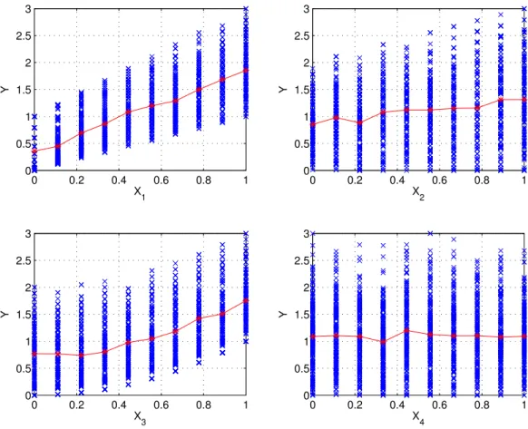
The correlation ratio is a useful estimator for input importance for general models. In addition, the scatter plots (the K plots, each with respect to individual inputs) from the replicated Latin hypercube samples provide useful visual information on how the output
0 0.2 0.4 0.6 0.8 1 0 0.5 1 1.5 2 2.5 3 X1 Y 0 0.2 0.4 0.6 0.8 1 0 0.5 1 1.5 2 2.5 3 X2 Y 0 0.2 0.4 0.6 0.8 1 0 0.5 1 1.5 2 2.5 3 X3 Y 0 0.2 0.4 0.6 0.8 1 0 0.5 1 1.5 2 2.5 3 X4 Y
Figure 1: An example scatter plot from replicated Latin hypercube sampling
behaves as Xi takes on different values Xij (for example, by inspecting the line joining the
means of all levels, namely, Xij’s in the Xi scatter plot.) In addition, when R is sufficiently
large (say, > 50), the parameter space is sufficiently explored so that the envelops encom-passing the output data in the scatter plots give additional qualitative information about parameter interactions (that Xi is interacting with some other inputs), although they
of-fer no additional information on which other inputs Xi interacts with (It requires two-way
interaction analysis described in Section 4 to quantify pair-wise interactions). An exam-ple is given in Figure 1 where the function is: Y = X1 +X1 ∗X2 +X32 with four inputs
Xi, i = 1,2,3,4;Xi ∈ [0,1]. Here, we observe in the scatter plots for X1 and X2 that the envelopes enclosing the data points are not uniform, indicating that these two input factors have interactions with other inputs. This observation agrees well with the example function. Furthermore, we observe thatX3 is nonlinear and X4 has negligible effect on the output.
4
An Improved Main Effect Analysis
To create a replicated Latin hypercube sample, both S (number of levels) and R (number of replications) have to be specified (such that N = SR) by users. In [14], McKay
investi-gated the variability of correlation ratio estimates as a function of sampling variability and concluded that sufficiency of the sampling design (specifically, S and R) is very important to achieve the desired precision. Specifically, largeN may be needed to adequately estimate the correlation ratios. In addition, if the biased correlation ratio estimator is used, large bias may result when R is small. Saltelli et al. [24] recommended that S should be larger than R to give good accuracy. Despite this recommendation, it should be noted that the adequacy of a sampling design is model dependent and thus not generally known a-priori. In this section we propose a more robust main effect analysis to address this issue.
Our improved main effect analysis is based on an iterative procedure consisting of an adaptive sampling scheme and an accuracy assessment tool to monitor the convergence of the correlation ratios. Our adaptive sampling scheme borrows from our earlier work on refinement of stratified designs [32]. Our improved method currently considers only adaptively increasing S (by a factor of 2 per refinement) for accuracy improvement while keeping R fixed. To offset the effect of bias [14], we use a moderate sized R and also the unbiased correlation ratio estimator.
In the rest of this section, we first show how to adaptively refine a replicated Latin hypercube design. We will then describe the iterative procedure utilizing this adaptive sampling scheme. A few examples will be given to study the effectiveness of this improved method.
4.1
Refinement for Replicated Latin Hypercube
We first denote a replicated Latin hypercube by an 3-tuple LH(N,K,S) whereN,KandSare the sample size, number of input parameters, and number of symbols or levels, respectively. The number of replications can be recovered by R = N/S. We begin with a fixed R (for example, R = 50) and an initial S (for example, S = 4). The basic idea in the refinement algorithm follows two major steps. The first step involves refining each grid cell (in a K -dimensional grid with S partitions in each dimension) into an 2K subgrid. Then for each
cell that already contains a sample point, a LH(2, K,2) (with size 2, K inputs, and 2 levels) containing the existing sample point is created for the grid cell. The refined sample can be shown to preserve its property as a replicated Latin hypercube. A selective random permutation is then applied to the newly created sample points to improve the statistical property of the entire refined sample while leaving the original sample points unchanged. The detailed refinement algorithm (Algorithm RefineLH) consists of the following steps (given an initial replicated LH sample matrix Z):
Pattern reconstruction: Transform the sample matrix Z (an N ×K matrix) to the corresponding LH pattern matrixAby (S is the current number of levels andR is the number of replications)
A(i, j) = d(Z(i, j)−Lj)/δXˆj)e, i= 1,· · ·, N;j = 1,· · ·, K,
Replication separation: Partition A into R individual LH pattern matrices Am, m =
1,· · ·, R (each Am is an S×K matrix). Then, for each Am,
Level refinement: Form another pattern matrix Bm (called base pattern matrix) from
Am by
Bm(i, j) = (dAm(i, j)e −1)∗2.
New sample insertion: Create the new pattern matrix ˜Am: for each row iof B,
1. Form a new LH pattern matrixCi of size 2×K.
2. SetCi ←Ci + [1 1]TBm(i),
3. PermuteCi to have one row matching Am(i) (by first exchanging entries of row 1
of Ci with entries in the same column so that row 1 matchesAm(i)).
4. Load ˜Am row 2×(i−1) + 1 to row 2×i with Ci.
Sample randomization: Perform random permutation to each column of ˜Am but only
to the newly created rows.
Sample concatenation: Append all ˜Am, m= 1,· · ·, R matrices to form the final ˜A
pat-tern matrix.
Sample Generation: Map the pattern matrix (which has number of levels = 2S now) to the new sample matrix ˜Z by scaling and translation with respect to the input ranges.
˜
Z(i, j) = ˜A(i, j)∗δXj+Lj+²(i, j)
where²(i, j) is a small random perturbation and its value depends on ˜A(i, j) to preserve the replicated LH property.
An example of refining a LH sample is given in [32].
4.2
An Adaptive Algorithm for Main Effect Analysis
The refinement technique can be used in an iterative procedure to improve the accuracy of main effect analysis. The algorithm is as follow:
1. Select an initial replicated LH sample with sample sizeN0 =S0R. Prescribe a precision 0< ² < 1. SetIteration = 0.
2. Set Iteration = Iteration + 1. Then evaluate the model using the current sample.
3. Use the sample inputs and outputs to compute the VCE’s.
4. If Iteration >1, do the following: for each VCE(Xi), compute the error ei by finding
5. If maxei < ², terminate.
6. Apply the Refine algorithmto create the refined LH sample. Then go to step 2. An alternative termination criterion for this procedure can be a prescribed maximum number of model evaluations. Using this criterion, the main effect analysis should give not only the VCE(Xi)’s, but also the estimated error bounds.
4.3
Numerical Results
In this section we demonstrate the effectiveness of our modified main effect algorithm on two test examples- one monotonic and one non-monotonic functions.
4.3.1 A Monotonic Test Problem
The first test problem is the monotonic Sobol’ function [24] given by:
Y = exp 6 X j=1 bjXj −I6 (10) whereb1 = 1.5, b2 =b3 =b4 =b5 =b6 = 0.9, I6 = 6 Y j=1 ebj−1 bj ,
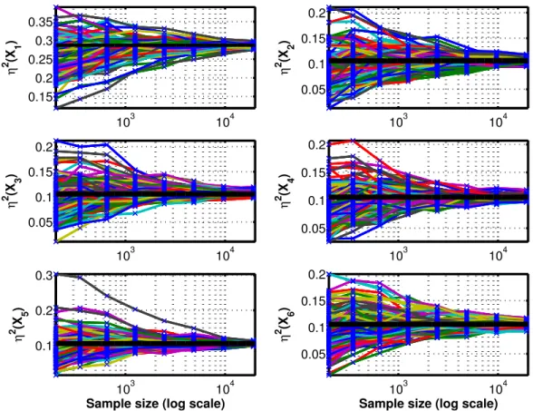
and Xj is uniformly distributed in [0,1]. The true correlation ratios for X1 is 0.287 and 0.1057 for Xj, j = 2,· · ·,6.
We simulate our iterative algorithm 100 times, each with an initial S of 4 and R = 50. Figure 2 shows the convergence history of the 6 correlation ratios as a function of S. Due to the randomness in the initial LH design and subsequent refinements, each of the 100 simulations goes through a different convergence path. The blue ’x’ in the plots are actual correlation ratios computed at different refinment levels. We observe firstly from the plots that all simulations exhibit similar paths converging to the true values as S is increased through refinement. In general, the spread of the correlation ratios shrinks asS is increased, demonstrating that larger sample sizes increase the confidence of the estimations. The reason that some envelopes expand a little initially is that the many sample point duplications due to the initial number of levels being too small (S = 4) limit the spread of the results.
4.3.2 A Non-monotonic Test Problem
The second test problem is the Ishigami function [24]:
103 104 0.15 0.2 0.25 0.3 0.35 η 2 (X 1 ) 103 104 0.05 0.1 0.15 0.2 η 2 (X 2 ) 103 104 0.05 0.1 0.15 0.2 η 2 (X 3 ) 103 104 0.05 0.1 0.15 0.2 η 2 (X 4 ) 103 104 0.1 0.2 0.3
Sample size (log scale)
η 2 (X 5 ) 103 104 0.05 0.1 0.15 0.2
Sample size (log scale)
η
2 (X
6
)
Figure 2: Sobol’ function: convergence history for the η2’s (black horizontal lines- true values)
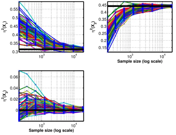
which has the following statistics ¯
Y = 3.5; V(Y) =π4/50 +π8/1800 + 1/2 + 49/8≈13.8445
η(X1) = 0.3139; η(X2) = 0.4424; η(X3) = 0.0
Again, We simulate our iterative algorithm 100 times, each with an initialSof 4 andR= 50. Figure 3 shows the convergence history of the 3 correlation ratios as a function ofS. Again, we observe that the correlation ratios converge to their true values asS is increased through refinement. We again observe that in general the spread of the correlation ratios in general shrinks asS is increased.
5
Two-way Interaction Analysis
In this section we extend the idea for main effect analysis to two-way interaction studies for uncorrelated inputs. In this case, we employ the following relationship
103 104 0.3 0.35 0.4 0.45 0.5 0.55 η 2 (X 1 ) 103 104 0.15 0.2 0.25 0.3 0.35 0.4 0.45
Sample size (log scale)
η 2 (X 2 ) 103 104 0 0.02 0.04 0.06
Sample size (log scale)
η
2 (X
3
)
Figure 3: Ishigami function: convergence history for the η2’s (black horizontal lines- true values)
where Xi and Xk are two distinct inputs under consideration. The first term on the right
hand side is the variance of the conditional expectation VCE(Xi, Xk) of Y, conditioned on
Xi and Xk. Again, the second term is the error or residual term measuring the estimated
variance of Y by fixing Xi and Xk. In addition, the correlation ratio for the input pair
(Xi, Xk) is
η2(Xi, Xk) =V(E(Y|Xi, Xk))/V(Y). (13)
A high correlation ratio shows thatXi and Xk taken together are important contributors to
the output variability. The variance due to the interaction term alone is defined as
V(Xi, Xk) =V(E(Y|Xi, Xk))−V(E(Y|Xi))−V(E(Y|Xk)). (14)
V(Xi, Xk) can be computed using many different techniques, for example, by directly
evaluating the corresponding integral. Here we illustrate its evaluation with the use of replicated orthogonal array sampling. Using orthogonal array design with a strength of 2,
Xi and Xk take on values Xij, j = 1,· · ·, S and Xkl, l = 1,· · ·, S where S is the number of
for any iand k in {1,· · ·, K}, i6=k, ¯ Y = 1 S2R s X j=1 S X l=1 R X r=1 Y(r)(X i =Xij, Xk=Xkl)), (15) and V(Y) = 1 SR S X j=1 S X l=1 R X r=1 h Y(r)(X i =Xij, Xk=Xkl)−Y¯ i2 , (16) where Y(r)(X
i = Xij, Xk = Xkl) is the output corresponding to Xi = Xij and Xk = Xkl
in the r-th replication (that is, keeping the two inputs at some fixed values and varying all others). The variance estimator for the expectation conditioned on Xi =Xij and Xk=Xkl
is ¯ Y(Xi =Xij, Xk =Xkl) = 1 R R X r=1 Y(r)(X i =Xij, Xk =Xkl) (17)
To approximate the variance of conditional expectation VCE(Xi, Xk), we use
VCE(Xi, Xk) = 1 S2 S X j=1 S X l=1 h ¯ Y(Xi =Xij, Xk =Xkl)−Y¯ i2 − (18) 1 S2R2 S X j=1 S X l=1 R X r=1 h Y(r)(Xi =Xij, Xk=Xkl)−Y¯(Xi =Xij, Xk =Xkl) i2 ,
and the two-way correlation ratio for input pair (i, k) is obtained by normalizing VCE(Xi, Xk)
with the output variance V(Y). Again, we can also compute the corresponding biased estimator by ignoring the second term in the above equation.
Finally, we arrive at the following pure two-way interaction effect
V(Xi, Xk) = VCE(Xi, Xk)−VCE(Xi)−VCE(Xk) (19)
where VCE(Xi) and VCE(Xi) can be obtained from the main effect analysis.
This same idea can be applied to the analysis of higher order interaction. For example, to analyze 3-way interaction, a replicated orthogonal array design of strength 3 can be used together with the corresponding formulas for computing the variance of conditional expectations.
5.1
An Improved Two-way Interaction Analysis
Our improved two-way interaction analysis is based on an iterative procedure consisting of an adaptive orthogonal array sampling scheme (based on our earlier work in [32]) and an accuracy assessment tool (similar to the one in our improved main effect analysis) to monitor the convergence of the correlation ratios. As opposed to replicated Latin hypercube designs which have a sample size growth factor of≈2 per refinement, the sample size growth factor
for orthogonal arrays isO(K2). Therefore, our improved procedure is less practical than the improved main effect analysis for large K (for example, K >5).
In the rest of this section, we first present the refinement algorithm for orthogonal arrays. We will then describe how to embed this refinement algorithm in the iterative procedure. A few examples will be given to study the effectiveness of our improved method.
5.2
Refinement for Replicated Orthogonal Arrays
We first denote a replicated orthogonal array by an 4-tuple OA(N,K,S,t) where N, K, S
andt are the sample size, number of parameters, number of symbols or levels, and strength, respectively. The number of replications can be recovered byR=N/(S2). We begin with a fixedR (for example, R = 50) and an initialS (the minimum S depends onK). The basic idea in the refinement algorithm is similar to that of the Latin hypercube and it consists of the following two steps: (1) refine each grid cell (in aK-dimensional grid withSpartitions in each dimension) into anSK subgrid; and (2) for each grid cell that already contains a sample
point, an OA(S2, K, S, t) including the existing sample point is created. The refined sample can be shown to preserve its property as a replicated orthogonal array. A selective random permutation is then applied to the newly created sample to improve the statistical property of the refined sample while leaving the original sample points unchanged. The refinement algorithm (Algorithm RefineOA) consists of the following steps:
Pattern reconstruction: same as in Algorithm RefineLH.
Replication separation: same as in Algorithm RefineLH.
Level refinement: For each pattern matrixAm, m= 1,· · ·, R, for another pattern matrix
Bm (called base pattern matrix) from Am by
Bm(i, j) = (dAm(i, j)e −1)∗2.
New sample insertion: Create the new pattern matrix ˜Am: for each row iof B,
1. Form a new OA pattern matrixCi with OA(S2, K, S,2).
2. SetCi ←Ci + [1 1]TBm(i),
3. PermuteCi to have one row matching Am(i) (by first exchanging entries of row 1
of Ci with entries in the same column so that row 1 matchesAm(i)).
4. Load ˜Am row S2×(i−1) + 1 to row S2×i with Ci.
Sample randomization: same as in Algorithm RefineLH.
Sample concatenation: same as in Algorithm RefineLH.
Sample Generation: same as in Algorithm RefineLH. An example of refining an OA sample is given in [32].
5.3
An Adaptive Algorithm for Two-way Interaction Analysis
The OA refinement technique can be used in an iterative procedure to improve the accuracy of interaction analysis. The algorithm is as follow:
1. Select an initial replicated OA sample with sample sizeN0 =S02R. Prescribe a precision 0< ² < 1. SetIteration = 0.
2. Set Iteration = Iteration + 1. Then evaluate the model using the current sample.
3. Use the sample inputs and outputs to compute the VCE’s.
4. If Iteration > 1, do the following: for each VCE(Xi, Xk), compute the error eik by
finding the difference between the current and the last VCE(Xi, Xk); else set eik =²..
5. If maxeik < ², terminate.
6. Apply the Refine algorithmto create a refined OA sample. Then go to step 2.
5.4
Numerical Results
In this section we demonstrate the effectiveness of our modified interaction analysis on two test examples- one monotonic and one non-monotonic functions.
5.4.1 A Monotonic Test Problem
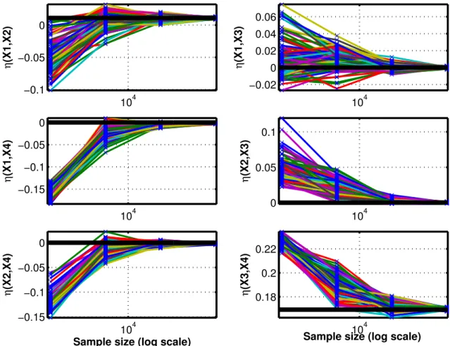
The first test problem is the following polynomial function given by:
Y =X1+X1X2+X3X43 (20) whereXj is uniformly distributed in [0,2].
We simulate our iterative algorithm 100 times, each with an initial S of 2 and R = 50. Figure 4 shows the convergence history of the 3 two-parameter correlation ratios as a function of N = S2R. Again, because of the randomness in the initial orthogonal array design and subsequent refinements, each of the 100 simulations goes through a different convergence path. We again observe that the correlation ratios of all 100 simulations converge to their true values asS is increased through refinement. In addition, the spread of the correlation ratios shrinks asS is increased, showing again that larger sample sizes increase the confidence of the estimations.
5.4.2 A Non-monotonic Test Problem
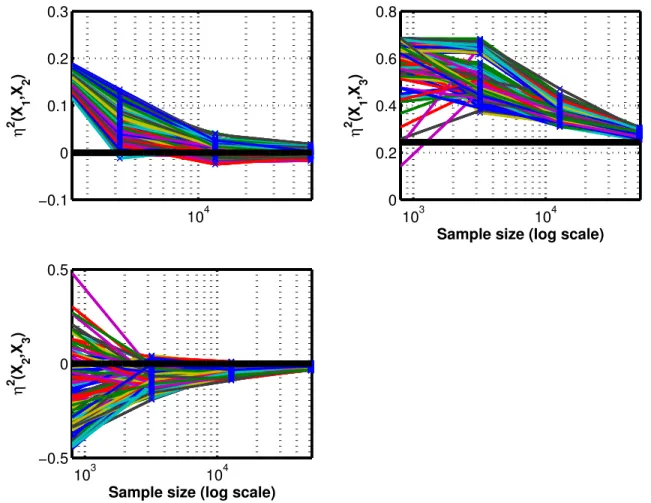
The second test problem is the Ishigami function [24]:
104 −0.1 −0.05 0 η (X1,X2) 104 −0.02 0 0.02 0.04 0.06 η (X1,X3) 104 −0.15 −0.1 −0.05 0 η (X1,X4) 104 0 0.05 0.1 η (X2,X3) 104 −0.15 −0.1 −0.05 0
Sample size (log scale)
η (X2,X4) 104 0.18 0.2 0.22
Sample size (log scale)
η
(X3,X4)
Figure 4: Polynomial function: convergence history for theη2’s (black horizontal lines- true values)
Once again we simulate our iterative algorithm 100 times, each with an initial S of 2 and
R = 50. Figure 5 shows the convergence history of the 3 two-way correlation ratios as a function ofS. Again, the same trends are observed as before.
6
Summary
In this paper we propose robust first- and second-order variance-based methods for global sensitivity analysis. Specifically, the use of refinement techniques in stratified sampling methods such as Latin hypercube and orthogonal array together with the corresponding analyses has enabled the accuracy assessment and improvement of the correlation ratios. We have demonstrated the effectiveness of these methods through a few numerical examples.
104 −0.1 0 0.1 0.2 0.3 η 2 (X 1 ,X 2 ) 103 104 0 0.2 0.4 0.6 0.8
Sample size (log scale)
η 2 (X 1 ,X 3 ) 103 104 −0.5 0 0.5
Sample size (log scale)
η
2 (X
2
,X 3
)
Figure 5: Ishigami function: convergence history for the η2’s (black horizontal lines- true values)
References
[1] F. Campolongo and R. Braddock, The use of graph theory in the sensitivity analysis of the model output: a new screening method, Reliability Engineering and System Safety 64 (1997), pp. 1-12.
[2] F. Campolongo, S. Tarantola, and A. Saltelli, Tackling quantitatively large dimension-ality problems, Computer Physics Communications 117 (1999) pp. 75-85.
[3] J. H. Friedman,Multivariate adaptive regression splines, Annals of Statistics19.1, 1-141, 1991.
[4] A. S. Hedayat, N. J. a. Sloane, and John Stufken, Orthogonal Arrays: Theory and Applications, Springer Series in Statistics, 1999.
[5] J. C. Helton and F.J. Davis, Latin Hypercube Sampling and the Propagation of Uncer-tainty in Analyses of Complex Systems,Reliability Engineering and System Safety, Vol. 81, No. 1, pp. 23-69, 2003.
[6] T. Homma and A. Saltelli, Importance measures in global sensitivity analysis of non linear models,Reliability Engineering and System Safety 52 (1996), pp. 117.
[7] T. Ishigami and T. Homma,An importance quantification technique in uncertainty anal-ysis for computer models, in Proceedings of the ZSUMA 90, University of Maryland, USA, 1990. p. 398403.
[8] R. L. Iman and W. J. Conover, A Distribution-free Approach to Inducing Rank Correla-tion Among Input Variables,Commun. Statist. Simula. Computa., Vol 11, pp. 311-334, 1982.
[9] J. Jacques and C. Lavergne, Sensitivity Analysis for Model with Correlated Inputs,
Reliability Engineering and System Safety 91 (2006), Issue 10-11, pp 1126-1134. [10] J. R. Koehler and A. B. Owen,Computer Experiments.
[11] T. Kolda, Revisiting Asynchronous Parallel Search for Nonlinear Optimization, Tech-nical Report SAND2004-8055, Sandia National Laboratories, Livermore, California, February 2004.
[12] T. J. Lorenzen and V. L. Anderson, Design of Experiments : A No-Name Approach,
Marcel Dekker, Inc. 1993.
[13] M. D. McKay, Evaluating Prediction Uncertainty, Los Alamos National Laboratory Technical Report NUREG/CR-6311, LA-12915-MS, 1995.
[14] M. D. McKay,Nonparametric Variance-based Methods of Assessing Uncertainty Impor-tance, Reliability Engineering and System Safety 57(1997), pp. 267-279.
[15] M. McKay, R. Beckman, W. Conover, A Comparison of Three Methods for Selecting Values of Input Variables in the Analysis of Output from a Computer Code, Techno-metrics, 21(2):239-245, 1979.
[16] M. McKay, M. A. Fitzgerald, and R. J.Beckman, Sample Size Effects when Using R2
to Measure Model Input Importance,LANL technical report.
[17] M. D. Morris, Factorial Sampling Plans for Preliminary Computational Experiments,
Technometrics, 21(2), pp. 239-245, 1991.
[18] M. D. Morris, Private communication via email.
[19] R. H. Myers and D. C. Montgomery, Response Surface Methodology, Second Edition, Wiley Series in Probability and Statistics, 2002.
[20] A. B. Owen,Orthogonal Arrays for Computer Experiments, integration, and visualiza-tion, Statist. Sinica 2, pp. 439-452, 1992.
[21] R. L. Plackett and J. P. Burman,The Design of Optimum Multifactorial Experiments,
Biometrika, 33, pp 305-325.
[22] M. Ratto, S. Tarantola and A. Saltelli,Estimation of Importance Indicators for Corre-lated Inputs,Proceedings of the European Conference on Safety and Reliability, ESREL 2001, E. Zio, M. Demichela, N. Piccinini (eds.), torino, 16-20 September 2001, vol. 1, pp. 157-164.
[23] A. Saltelli,Making best use of model evaluations to compute sensitivity indices,Comput. Phys. Commun. 145 (2002), pp. 280297.
[24] A. Saltelli, K. Chan, E. M. Scott (editors),Sensitivity Analysis,Wiley Series in Proba-bility and Statistics, 2000.
[25] I. M. Sobol, Sensitivity estimates for nonlinear mathematical models, Mathematical modeling and computational experiments, 1993.
[26] A. Saltelli, S. Tarantola, and K. Chan, A Quantitative Model-Independent Method for Global Sensitivity Analysis of Model Output, Technometrics, Vol. 41, No. 1, pp. 39-55, 1999.
[27] A. Saltelli, S. Tarantola, F. Campolongo, and M. Ratto,Sensitivity Analysis in Practice,
Wiley, 2004.
[28] M. Stein, Large Sample Properties of Simulations Using Latin Hypercube Sampling,
Technometrics, 29(2), pp. 143-151.
[29] B. Tang,Latin Hypercubes and Supersaturated Designs, Dissertation, Dept. of Statistics and Acturial Science, University of Waterloo, 1992.
[30] B. Tang, Orthogonal Array-based Latin Hypercubes, J. Amer. Statist. Assn. 88, 1392-1397, 1993.
[31] S. Tarantola,Quantifying uncertainty importance when Inputs are correlated,Foresight and Precaution, edited by Cottam, Harvey, Pape and Tait (eds), pp. 1115-1120, 2000. [32] C. Tong,Refinement Strategies for Stratified Sampling Methods,Reliability Engineering
and System Safety 91 (2006), Issue 10-11, pp 1257-1265.
[33] C. Tong and F. Graziani, A Global Sensitivity Analysis Methodology for Multi-physics Applications, LLNL Technical Report UCRL-TR-227800, 2007.