Statistical methods for
QTL mapping and genomic prediction of
multiple traits and environments:
case studies in pepper
Thesis committee Promotor
Prof. Dr F.A. van Eeuwijk Professor of Applied Statistics Wageningen University
Co-promotor Dr M.C.A.M. Bink
Senior Quantitative Geneticist
Hendrix Genetics - Research & Technology Centre, Boxmeer
Other members
Prof. Dr R.F. Veerkamp, Wageningen University Prof. Dr P.C. Struik, Wageningen University Dr R. Rincent – INRA Clermont Ferrand, France Dr E.J. Gutteling, Rijk Zwaan, Fijnaart
This research was conducted under the auspices of the Graduate School for Production Ecology & Resource Conservation (PE-RC).
QTL mapping and genomic prediction of
multiple traits and environments:
case studies in pepper
Nurudeen Adeniyi ALIMI
Thesis
submitted in fulfilment of the requirements for the degree of doctor at Wageningen University
by the authority of the Rector Magnificus Prof. Dr A.P.J. Mol,
in the presence of the
Thesis Committee appointed by the Academic Board to be defended in public
on Tuesday 1 November 2016 at 1.30 p.m. in the Aula.
Nurudeen Adeniyi ALIMI
Statistical methods for QTL mapping and genomic prediction of multiple traits and environments: case studies in pepper
165 pages.
PhD thesis, Wageningen University, Wageningen, NL (2016) With references, with summary in English
ISBN: 978-94-6257-936-1
To the past -
Maami and Magaji
The present –
’Mobola and Kiyaan
In this thesis we describe the results of a number of quantitative techniques that were used to understand the genetics of yield in pepper as an example of complex trait measured in a number of environments. Main objectives were; i) to propose a number of mixed models to detect QTLs for multiple traits and multiple environments, ii) to extend the multi-trait QTL models to a multi-trait genomic prediction model, iii) to study how well the complex trait yield can be indirectly predicted from its component traits, and iv) to understand the ‘causal’ relationships between the target trait yield and its component traits.
The thesis is part of an EU-FP7 project “Smart tools for Prediction and Improvements of
Crop Yield” (SPICY- http://www.spicyweb.eu/). This project generated phenotypic data from four environments using 149 individuals from the sixth generation of recombinant inbred
lines obtained from intraspecific cross between large –fruited inbred pepper cultivar ‘Yolo
Wonder’ (YW) and the hot pepper cultivar ‘Criollo de Morelos 334’ (CM 334). A total of 16 physiological traits were evaluated across the four trials and various types of genetic parameters were estimated. In a first analysis, the traits were univariately analyzed using
linear mixed model. Trait heritabilities were generally large (ranging between 0.43 – 0.96
with an average of 0.86) and mostly comparable across trials while many of the traits displayed heterosis and transgression. The same QTLs were detected across the four trials, though QTL magnitude differed for many of the traits. We also found that some QTLs affected more than one trait, suggesting QTL pleiotropy (a QTL region affecting more than one trait). We discussed our results in the light of previously reported QTLs for these and similar traits in pepper.
We addressed the presence of genotype-by-environment interaction (GEI) in yield and the other traits through a multi-environment (ME) mixed model methodology with terms for QTL-by-environment interaction (QEI). We opined that yield would benefit from joint analysis with other traits and so deployed two other mixed model based multi-response QTL approaches: a multi-trait approach (MT) and a multi-trait multi-environment approach (MTME). For yield as well as the other traits, MTME was superior to ME and MT in the number of QTLs, the explained variance and accuracy of predictions. Many of the detected QTLs were pleiotropic and showed quantitative QEI. The results confirmed the feasibility and strengths of novel mixed model QTL methodology to study the architecture of complex traits. The QTL methods considered thus far are not well suited for prediction purposes as only a limited set of QTL-related markers are used. Since the main interest of this research includes improvement of yield prediction, we explored both single-trait and multi-trait versions of genomic prediction (GP) models as alternatives to the QTL-based prediction (QP) models. This was termed direct prediction. The methods differed in their predictive accuracies with GP methods outperforming QP methods in both single and multi-traits situations. We borrowed ideas from crop growth model (CGM) to dissect complex trait yield into a number of its component traits. Here, we integrated QTL/genomic prediction and CGM approaches and showed that the target trait yield can be predicted via its component traits together with environmental covariables. This was termed indirect prediction. The CGM approach seemed
strongly driven by just one of its components, the partitioning to fruit.
An alternative representation of the biological knowledge of a complex target trait such as yield is provided by network type models. We constructed both conditional and unconditional
networks across the four environments to understand the ‘causal’ relationships between target
trait yield and its component traits. The final networks for each environment from both conditional and unconditional methods were used in a structural equation model to assess the causal relationships. Conditioning QTL mapping on network structure improved detection of refined genetic architecture by distinguishing between QTL with direct and indirect effects, thereby removing non-significant effects found in the unconditional network and resolving QTL pleiotropy. Similar to the CGM topology, yield was established to be downstream to its component traits, indicating that yield can be studied and predicted from its component traits. Thus, the genetic improvements of yield would benefit from improvements on the component traits.
Finally, complex trait prediction can be enhanced by a full integration of the methods described in the different chapters. Recent research efforts have been channelled to incorporating both multivariate whole genome prediction models and crop growth models. Further research is required, but we hope that the present thesis presents useful steps towards better prediction models for complex traits exhibiting genotype by environment interaction.
Table of Contents
Abstract ... vi
Table of Contents ... viii
1. General Introduction ... 1 2. General Introduction ... 3 1.1. Background ... 3 1.2. Mapping Populations ... 4 1.3. Mapping Techniques ... 4 1.3.1. ANOVA model ... 5
1.3.2. Interval Mapping/Mixture model ... 5
1.3.3. Multiple Linked QTLs ... 5
1.3.4. (Multivariate) Multiple Regression ... 6
1.3.5. Mixed Model ... 6
1.3.6. Probabilistic Models Based on Bayesian Theory ... 7
1.4. Genomic Prediction Models ... 8
1.5. Phenotype Network Models ... 9
1.6. QTL by Environment Interaction ... 10
1.7. QTL mapping in Pepper ... 10
1.8. Overview/Outline of this thesis ... 11
Genetic and QTL analyses of yield and a set of physiological traits in pepper ... 13
3. Genetic and QTL analyses of yield and a set of physiological traits in pepper ... 15
2.1. Abstract ... 15
2.2. Introduction ... 16
2.3. Materials and Methods ... 17
2.3.1. Plant materials ... 17
2.3.2. Phenotyping experiments and designs ... 17
2.3.3. Trait evaluation ... 18
2.3.4. Phenotypic analysis ... 19
2.3.5. Marker data and Linkage map ... 20
2.3.6. QTL estimation ... 21
2.4. Results ... 22
2.4.1. Traits evaluation ... 22
2.4.2. Heritability & genetic correlation ... 23
2.4.3. QTL results ... 25
Appendix 2A: EU-SPICY Experimental set-up ... 33
Appendix 2B: Phenotypic Mean comparison ... 35
4. Multi-Trait and Multi-Environment QTL Analyses of Yield and A Set of Physiological Traits in Pepper ... 37
5. Multi-Trait and Multi-Environment QTL Analyses of Yield and A Set of Physiological Traits in Pepper ... 39
3.1. Abstract ... 39
3.2. Introduction ... 40
3.3. Materials and Methods ... 41
3.3.1. Plant materials, marker data and phenotypic evaluation ... 41
3.3.2. Multi-environment phenotypic and QTL analysis ... 42
3.3.3. Multi-trait QTL estimation ... 43
3.3.4. Multi-Traits Multi-Environments QTL estimation ... 44
3.3.5. MTME final QTL selection and window size ... 44
3.3.6. Comparisons of ME, MT and MTME approaches ... 45
3.4. Results ... 45
3.4.1. Genetic correlations between traits (within and between trials) ... 45
3.4.2. Multi-Environment analyses ... 45
3.4.3. Multi-trait analyses ... 46
3.4.4. Multi-trait multi-environment analysis ... 48
3.4.5. Comparison of MT, ME, and MTME results ... 49
3.5. Discussion ... 55
Appendix 3A: Traits Description ... 59
Appendix 3B: Biplots for BLUEs and fitted trait values ... 60
Appendix 3C: QTL by Environment Results from the ME analyses ... 60
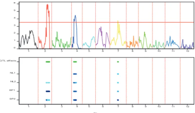
Appendix 3D: QTL Effects from the MT analyses ... 64
Appendix 3E: QTL Effects from the MTME analyses: Chromosomes 3-12 ... 66
4. Predicting complex traits in multiple environments by a combination of genomic prediction and crop growth modelling: an example in pepper ... 71
8. Predicting complex traits in multiple environments by a combination of genomic prediction and crop growth modelling: an example in pepper ... 73
4.1. Abstract ... 73
4.2. Introduction ... 74
4.3. Materials and Methods ... 76
4.3.1. Genotypic and Phenotypic data ... 76
4.3.2. Univariate and Multivariate QTL Prediction Models ... 76
4.3.5. Multivariate Genomic Prediction Model: Bayesian Latent Variable ... 78
4.3.6. Yield Indirect Prediction through Crop Growth Model ... 79
4.3.7. Model Validation and Accuracy... 80
4.3.8. Yield Prediction Strategies ... 81
4.4. Results ... 82
4.4.1. Trait Descriptions ... 82
4.4.2. Predictive Ability and Bias of the Four Prediction Models ... 82
4.4.3. Accuracies of Yield Prediction from Crop Growth Model ... 85
4.5. Discussion ... 88
5. A network analysis of yield and yield components across environments: an example in pepper ... 93
6. A network analysis of yield and yield components across environments: an example in pepper ... 95
5.1. Abstract ... 95
5.2. Introduction ... 96
5.3. Materials and Methods ... 97
5.3.1. Genotypic and Phenotypic data ... 97
5.3.2. Traits Relationships from Crop Growth Model ... 98
5.3.3. Unconditional Network (MTM) ... 98
5.3.4. Conditional Network (QTLnet) ... 99
5.4. Results ... 101 5.5. Discussion ... 107 Appendix 5A ... 110 Appendix 5B ... 111 6. GENERAL DISCUSSION ... 113 7. GENERAL DISCUSSION ... 115 6.1. Introduction ... 115 6.2. Mapping Population ... 116 6.3. QTL mapping resolution ... 118
6.4. Manual and Automated Phenotyping ... 119
6.5. Complex Traits Analyses ... 120
6.5.1. QTL methods based on linear mixed model ... 121
6.5.2. Genomic Prediction and Integrated Crop Growth Models ... 126
6.5.3. Causal network model ... 129
6.6. Concluding Remarks ... 131
References ... 133
Curriculum Vitae ... 151 Publication List ... 152 PE&RC Training and Education Statement ... 153
CHAPTER 1
CHAPTER 1
2.
General Introduction
1.1.
Background
The production of genetically improved crop cultivars capable of satisfying human requirements such as yield, quality, tolerance to certain environmental conditions and disease resistance has always been the main challenge for plant breeders. The breeder must identify and select superior genotypes capable of conferring the desired requirement(s) on the plant. This is a result of often complex genetics that underlie the expression of most of the economically important traits. Since most of the observable phenotypic variations between individual plants from the same species are quantitative, the development and application of quantitative genetics theory in the last century has greatly improved the understanding of the genetic basis of complex traits. In quantitative genetics, the genetic architecture of a quantitative trait is described with the aid of an underlying genetic model. Variation in (complex) quantitative traits is caused by segregation at multiple loci with individually small effects (polygenic) that may be sensitive to the environment (Mackay, 2001). For such complex traits, the quantitative trait loci (QTL) genotypes cannot be determined from segregation of phenotypes in controlled crosses or pedigrees because the relationship between genotype and phenotype is not a simple ratio.
Until recently, the understanding of complex traits has been developed without having direct access to the DNA, the place where the QTLs responsible for genetic variation ultimately reside. The availability of marker genotyping that provide information directly related to the DNA opened new possibilities for the further development of genetic models that included explicit representations of the hereditary material. With molecular genetics, it is expected that information at the DNA level will lead to faster genetic gain than that achieved based on phenotypic data only. The application of molecular markers has enabled the dissection of complex traits into the underlying QTLs. These molecular markers do exhibit Mendelian segregation (Uptmoor et al., 2008). The increasing knowledge on QTLs for important agronomic traits gives new opportunities in marker-assisted selection (MAS) (Ribaut and Hoisington, 1998; Uptmoor et al., 2008). The use of these molecular breeding techniques has considerably contributed to unravel crop traits affecting quality and yield of plant products and to gain insight into their genetic basis. The basic principle behind the use of MAS in the
context of QTL mapping can be expressed as: If a QTL is linked to a marker locus, there will
be a difference in mean values of the quantitative trait among individuals with different
genotypes at the marker locus (Sax, 1923). Among the most popular types of molecular
markers employed in QTL mapping are Restriction Fragment Length Polymorphisms (RFLP) (Beckmann and Soller, 1986; Tanksley et al., 1989), Simple Sequence Repeats (SSR) (Powell et al., 1996), Amplified Fragment Length Polymorphisms (AFLP) (Vos et al., 1995) and Single-Nucleotide Polymorphism (SNP) (Syvänen, 2005). Each molecular marker system has
its own advantages and disadvantages (Semagn et al., 2006), the focus of which is not within the scope of this work. Nowadays genomes have been sequenced and commercial SNP arrays are available for many field and horticultural crops which makes genome-wide genotyping affordable.
1.2.
Mapping Populations
The types of populations most commonly used for QTL mapping are segregating populations
originating from crosses between inbred lines such as F2, backcross, or recombinant inbred
line (RIL). This is mainly due to the possibility of producing relatively large populations with known genetic structure, as there are only two founder genotypes (Robertson, 1967). These population types have been in use long before the advent of molecular markers. Decisions on selection of parents and mating design for development of mapping population and the type of markers used depend upon the objectives of experiments, availability of markers and the molecular map. The parents of mapping populations must have sufficient variation for the traits of interest at both the DNA sequence and the phenotype level. The variation at DNA level is essential to trace the recombination events. The more DNA sequence variation exists, the easier it is to find polymorphic informative markers. When the objective is to search for genes controlling a particular trait, genetic variation of trait between parents is important. If the parents are greatly different at phenotypic level for a trait, there is a reasonable chance that genetic variation exists between the parents, although uncontrolled environmental effects could create large phenotypic variation without any genetic basis for the effects. However, lack of phenotypic variation between parents does not mean that there is no genetic variation, as different sets of genes could result in same phenotype (Mackay, 2001; Ribaut and Hoisington, 1998). Other types of population used in plant breeding include pedigree population (Bink et al., 2002; Rosyara et al., 2009), association panels (Jannink and Walsh, 2002) and Multi-parent Advanced Generation Inter-Cross (MAGIC) population (Cavanagh et al., 2008; Huang et al., 2012).
1.3.
Mapping Techniques
Before the development of mapping techniques, the knowledge about the genetic architecture of quantitative traits was limited to estimates of trait heritability and other variance components derived from correlations between relatives and response to selection, estimates of average degree of dominance from changes of mean on inbreeding, estimates of net pleiotropic effects from genetic correlations, and estimates of the total mutation rate from phenotypic divergence between inbred lines. There was the need to go beyond these mere statistical descriptions in order to more effectively select domestic crop species for improved production traits, and understand the genetic basis of adaptation (Mackay, 2001). The need to identify and determine the properties of the individual genes underlying variation in complex traits (Jannink et al., 2001) led to increasing improvements in statistical techniques for QTL mapping, and experimental design.
Within the last two decades, many QTL mapping methods have been developed either based on least square (LS) or maximum likelihood (ML) estimation and recently based on Bayesian paradigm. LS methods test for differences in means between marker class using either
ANOVA or regression (Soller et al., 1976), while ML uses full information from the marker-trait distribution, and explicitly accounts for QTL data being mixtures of normal distributions. Each of these estimation techniques come with their advantages and disadvantages. However there is, in general, little difference in power between the two techniques (Haley and Knott, 1992; Lander and Botstein, 1989a) and ML interval mapping can be approximated using regressions (Haley and Knott, 1992; Martinez and Curnow, 1992).
1.3.1. ANOVA model
This is the most basic form of QTL mapping comparing the means of the marker genotypes for individual marker loci, under the hypothesis that the marker loci coincide with a QTL (Soller et al., 1976). The marker genotypes define the levels of a treatment factor, an analysis of variance is then performed and marker-trait associations tested using standard F-tests. This model can be easily extended to accommodate QTL interactions and fixed effects. A major drawback is that assumptions of homogeneity (perfect linkage disequilibrium) may be violated. QTL effect and QTL location may be confounded in terms of distance to the marker i.e. a closely linked QTL with a moderate allele effect and a major QTL that is loosely linked will produce a comparable test statistic for marker-trait association.
1.3.2. Interval Mapping/Mixture model
In 1989, Lander and Botstein (Lander and Botstein, 1989a) proposed the use of genetic map information to overcome the limitation of the individual marker approach in a strategy called interval mapping (IM) using ML estimation. ML estimates for the model parameters are obtained with the assumption that observations are from a mixture of normal distributions (one distribution per QTL genotype class). Though the QTL genotypes are unknown in between markers, the flanking markers can be used to infer conditional probabilities for the QTL genotypes given the flanking marker genotypes and the recombination frequencies between the QTL and the markers. The conditional probabilities for the QTL genotypes are then used as mixing proportions in the calculation of the likelihood for the mixture model. Likelihood ratio (LR) test is performed to determine whether the phenotypic data support a mixture distribution, i.e., the presence of a QTL at the evaluation position in the genome. Typically, the log-likelihood ratio (LLR), or LOD score (= LLR/4.61) is plotted along the genome as a profile.
1.3.3. Multiple Linked QTLs
The presence of multiple linked QTLs biases both single marker and interval mapping analysis (Knott and Haley, 1992), and segregation of unlinked QTLs inflates the within-marker class phenotypic variance, thus reducing the power of QTL detection. This led to further improvements to the IM approach through composite interval mapping (CIM) (Jansen and Stam, 1994; Zeng, 1994) and multiple interval mapping (MIM) (Kao et al., 1999). Composite interval mapping (CIM) combines ML interval mapping with multiple regression, using marker cofactors to reduce the bias in estimates of position and effects of QTLs introduced by multiple linked QTLs. CIM also leads to an increase in QTL detection power since the within marker-class phenotypic variation is decreased. Strictly speaking, CIM
methods are not multiple QTLs methods, in that the model for evaluating the effects of each interval depends on the marker cofactors included, which varies across intervals (Mackay, 2001). Multiple interval mapping (MIM) is a true multiple QTLs method. It converges to a stable model providing estimates of positions and main and interaction effects of multiple QTLs (Kao et al., 1999). It should be noted that in CIM and MIM methods, estimates of QTL positions and effects are highly model dependent, and can vary given different numbers of marker cofactors and window sizes (the region to either side of the test interval within which no marker cofactors are fitted) (Pasyukova et al., 2000; Zeng et al., 1999; Zeng, 1994). These factors are under the control of the researcher, who must bear in mind that the model with the best fit and the the highest number of identified QTLs, is not necessarily the closest approximation to reality (Mackay, 2001).
1.3.4. (Multivariate) Multiple Regression
With more than one QTL, the use of mixture models becomes computationally intensive and less versatile. The use of multiple regressions QTL mapping approach was therefore proposed as a more efficient and computationally less intensive alternative. The regression approach has been shown to produce very similar results to the mixture model strategy (Haley and Knott, 1992; Kao, 2000) and can be implemented within standard statistical packages. Regression can also be employed for a complex data structure having QTL and multi-environment, with possibility to model QTL by environment interaction (Jiang and Zeng, 1995; Sari-Gorla et al., 1997).
Extensions to the multi-trait case have been proposed for both mixture and regression based models (Hackett et al., 2001; Jiang and Zeng, 1995; Knott and Haley, 2000). CIM was extended to multiple traits, enabling the evaluation of the main QTL effects as well as pleiotropy and QTL by environment interactions (Jiang and Zeng, 1995). The multi-trait extension of regression based framework was also proposed and implemented (Hackett et al., 2001; Knott and Haley, 2000). Multivariate multiple regression approaches do show greater flexibility than mixture models in extensions to account for additional treatment and block structure, they are not yet robust enough to account for commonly encountered complications as imbalance and complex error structures (Malosetti, 2006).
1.3.5. Mixed Model
Some of the issues in QTL detection and analyses involve the underlying design of the phenotypic experiment which may induce unequal replication of genotypes (unbalanced) and/or measurements over time (repeatedness). Also, most of the experiments involve collections of genotypes evaluated for multiple traits across multiple environments. It is also possible that the relationship between measured traits and explanatory variables such as genotype and environment characterizations is not well captured by a linear assumption. Mixed models (Verbeke and Molenberghs, 2000) offer a suitable framework to jointly analyse such data without imposing unrealistic assumptions, such as zero genetic correlations between environments and traits, and constant variance across environments. Mixed model is also capable of accounting for possible unbalanced design setting and repeatedness. They can account for both intra- and inter-trial variability in the estimation of QTL effects and trait
values prediction and facilitate the representation of genetic relationship among related lines thereby offering a condition for valid inference on QTLs (Van Eeuwijk et al., 2010). The linear assumption can be relaxed and the relationship modelled by non-linear functions with inclusion of growth parameters thereby mimicking eco-physiological models. Mixed model can be applied to several settings commonly found in plant breeding experiments. The simplest of such settings is single-trait-single-environment which can be extended up to the most complex setting of multi-trait (possibly correlated) multi-environment setting with various interactions (traits, environments and/or environmental characterization). Most of these settings with several structures for expectations, correlations and variance-covariance have been analysed in literature.
1.3.6. Probabilistic Models Based on Bayesian Theory
Most genetic properties of plants and animals, individuals, populations or species are a product of processes that are inherently stochastic and are mostly interdependent. Therefore, they are better studied using probabilistic models. In the Frequentist approach, probability is viewed from the framework of hypothetically repeating an experiment many times under identical circumstances. In the Bayesian approach, a probability is a direct measure of uncertainty, and might or might not represent a long-term frequency. Bayesian and Frequentist statistics aim at making inferences about a fixed, but unknown, parameter value but they differ in approach and in interpretation of the results. Bayesian analysis incorporates background (prior) information into the specification of the model. This prior information is combined with information from the data (likelihood) to generate the posterior distribution over the parameter values, according to Bayes’ rule. The choice of prior information can be based on previous experiments, experts input, theoretical or other considerations. Bayesian methods can be especially valuable in complex problems or in situations that do not conform naturally to a classical setting. Many genetics problems fall into one of these categories (Shoemaker et al., 1999). In addition, Bayesian approaches can be easier to interpret. The paper of Beaumont and Rannala (2004) reviewed the application of Bayesian inference in some areas of genetics including population genetics, genomics and human genetics with specific reference to analysis of complex trait, linkage mapping and QTL mapping. In QTL analyses, inference is typically concerned with identifying those loci on the genome that contribute significantly to the quantitative trait of interest. Through Bayesian approach, the probability that a locus positioned near a known molecular marker has a genotype directly associated with the trait can be calculated and the QTLs which directly influence the trait can be identified.
The Bayesian approach has been successfully applied in a wide range of applications. Bayesian analysis based on QTL intensity has been proposed for obtaining posterior modes and credibility intervals for the QTLs (Sillanpää and Arjas, 1998). Various Bayesian techniques for handling complex plant and animal pedigreed populations have been suggested and implemented. Sisson and Hurn (2004) discussed existing approaches to the use of Bayesian model in making inference on QTLs and suggested a modification to the loss function for estimating both the number of QTL and their location. Bauer et al. (2009) developed a Bayesian multi-locus multi-environmental method of QTL analysis. Through a
real life data and simulation study, the strategy was compared to (a) Bayesian multi-locus mapping, where each environment is analyzed separately, (b) Restricted Maximum Likelihood (REML) single-locus method, using a mixed hierarchical model, and (c) REML forward selection applying a mixed hierarchical model.
Just as in regression analysis, model selection can also be handled within the Bayesian framework. Here, the model selection problem is transformed to the form of parameter estimation. Several Bayesian model selection methods have been developed among which are Kuo & Mallick, Gibbs Variable Selection (GVS), Stochastic Search Variable Selection (SSVS), adaptive shrinkage and model space approach (reversible jump MCMC and composite model space) (O'Hara and Sillanpää, 2009). Yi et al., (2007) extended the Bayesian model selection framework they earlier proposed for mapping epistatic QTLs in experimental
crosses to include environmental effects and gene–environment interactions. A new fast
Markov chain Monte Carlo algorithm was proposed to explore the posterior distribution of unknowns. In addition, this takes advantage of any prior knowledge about genetic architecture to increase posterior probability on more probable models.
1.4.
Genomic Prediction Models
The availability of genome-wide dense marker maps at affordable cost have made the use of genomic selection (GS) models an interesting alternative to marker-assisted models. GS models predict the genetic value of selection candidates based on the genomic estimated breeding value (GEBV) predicted from high-density markers positioned throughout the genome. Unlike marker-assisted selection, the GEBV is based on all markers including both minor and major marker effects. Thus, the GEBV may capture more of the genetic variation for the particular trait under selection. The GS models have become the standard methods for predicting genetic values in animals (De Los Campos et al., 2009; Goddard and Hayes, 2009) and also recently in plants (Crossa et al., 2010; Heslot et al., 2012; Jannink et al., 2010). GS models can be based on either Frequentist or Bayesian paradigm. Unlike QTL-based models where selected markers are used, in the GS models, all markers are used in a penalized regression context for prediction.
The key principle of GS is to simultaneously estimate the effects of all genome-wide markers in a training population consisting of genotyped and phenotyped individuals and then predict the genomic estimated breeding value (GEBV) of genotyped but not-phenotyped individuals in test/future generations (Meuwissen et al., 2001). GEBVs are calculated as the sum of estimated marker effects for genotyped individuals in a training population. Fitting all markers simultaneously ensures that marker-effect estimates are unbiased, small effects are captured, and there is no multiple testing issue (Jia and Jannink, 2012). Due to the usually large number of markers relative to number of individuals, variable selection and shrinkage estimation methods are employed to tackle the problem of high dimensionality in the predictors (De Los Campos et al., 2009; Habier et al., 2011; Hayes et al., 2009; Legarra et al., 2011). These estimation methods try to reduce mean squared error (MSE) by reducing the variance of the estimator. This may however introduce bias in the estimate. The obtained penalized estimates are the solution to an optimization problem that balances model fit and
model complexity. Both parametric and semi-parametric GS methods have been proposed to handle the problem of high dimensionality and other peculiar issues including markers colinearity. Some example of GS methods include ridge regression (Hoerl and Kennard, 1970), Least Absolute Shrinkage and Selection Operator (LASSO) (Tibshirani, 1996), Bayes A and Bayes B of Meuwissen et al. (2001) and the Bayesian LASSO (Park and Casella, 2008), reproducing kernel Hilbert spaces (RKHS) regression (Gianola and van Kaam, 2008). Evaluations and comparisons of performances of a number of GS models in plant breeding is presented in Heslot et al. (2012).
1.5.
Phenotype Network Models
Understanding the interconnectedness among plant phenotypes has become a key objective in QTL mapping. The vast opinions in recent literature advocate for the need to study how plant phenotypes are interconnected in networks of dependencies and the stability of the relationships across environments due to genotype-by-environment interactions (Granier and Vile, 2014; Li et al., 2010; Valente et al., 2013). Complex traits are often associated with multiple correlated traits referred to as component traits. Physiological interactions among target and component traits, together with shared genetic factors may be responsible for observed associations among these traits (Li et al., 2006). The genetic improvements of a complex target trait would benefit from improvements on the component traits, especially when the mechanism of (causal) association between the target and component traits is known. Although traditional multi-trait models are able to account for covariations among traits and establish QTLs with pleiotropic effects, they are not able to disentangle the paths for such effects neither are they able to provide insight into the (causal) relationships among the traits. Properly studying the interconnectedness will reveal causal relationship among phenotypes.
Causal inference methodology was introduced as early as the 1921 (Wright, 1921). The methods have been further developed and applied since then in genetics and other fields (Spirtes et al., 2000). Incorporating QTLs in network models has been shown to facilitate causal inference (Li et al., 2006; Neto et al., 2008), enabling differentiation of QTL effects on phenotypes into direct and indirect effects. QTLs in network models also provide an intuitive explanation for pleiotropic QTLs and possible QTL hotspots region where a QTL influences many traits. Graphical models with arrows pointing in the direction of causality are often used to depict the inferred relationship (Neto et al., 2010). However, causality claim cannot be established from data alone. Some assumptions about the causal relationships among the variables being modelled are needed. In genomic network studies, causality claim stems from two facts. First is the analogy between randomized experimental design and genetic randomization that occurs during meiosis. Second is the intuition that phenotypic variation is caused by genetic factors (Li et al., 2006; Neto et al., 2010). Relying solely on correlation between traits to claim causality is not enough even when the traits share a common QTL. Understanding biological reasoning governing the relationship is crucial (Li et al., 2010).
1.6.
QTL by Environment Interaction
Yield as an example of complex quantitative traits of plants measured on collections of genotypes across multiple environments is the result of processes that depend simultaneously on genotype and environment in intricate ways (Boer et al., 2007). For complex traits that exhibit considerable genotype by environment interaction, these QTLs have to be analyzed by considering the combination of the QTLs under different environment using QTL x E analysis (Ribaut and Hoisington, 1998; Slafer, 2003). An overview of the state of the art in QTL analyses and crop performance under environmental conditions is provided in the review by Collins et al. (2008). The improvement of crop yield has been possible through the indirect manipulation of QTLs that control heritable variability of the traits and physiological mechanisms that determine biomass production and its partitioning. Also, most QTLs are not stable across environments. QTLs can therefore be categorized according to the stability of their effects across environmental conditions. A ‘constitutive’ QTL is consistently detected across most environments, while an ‘adaptive’ QTL is detected only in specific environmental conditions or increases in expression with the level of an environmental factor e.g. a QTL that is expressed more strongly with increasing temperature (Vargas et al., 2006). The magnitudes of these adaptive QTLs, therefore, vary greatly between experiments.
Further, complex agronomic traits such as yield have low heritability, are strongly dependent on environmental changes and show high genotype by environment interactions (GEI) (Tardieu, 2003). The genetic analysis of such highly variable traits needs a strategy to cope with the temporal variability of phenotypes. Physiological models could help in understanding GEI interactions and speed up crop improvement for targeted environments (Boote et al., 2001; MAYES et al., 2005; Slafer, 2003). One strategy involves interpreting networks of field trials using a statistical method that calculates QTL x E interactions (Malosetti et al., 2006). Another strategy known as eco-physiological model involves modelling the measured traits by an underlying physiological model of which several non-genetic input variables closely describe the characteristics of the environments (Marcelis et al., 2006; Tardieu, 2003).
1.7.
QTL mapping in Pepper
Pepper, a member of the Solanaceae family, is a naturally self-pollinating warm season
perennial with expected lifespan of about 20 years. It is diploid with 12 chromosome pairs.
Most pepper species originated from South America (DeWitt and Bosland, 1996). Capsicum
annuum, which is the most commercially important and most widely cultivated species
worldwide, is used in this study. A number of studies have reported on genetic parameters of a series of pepper traits and performed QTL mapping for these traits. Among pepper traits
already studied are those related to disease resistance (Lefebvre and Palloix, 1996; Caranta et
al., 1997a), and sensory traits such as pungency (Blum et al., 2003; Ben Chaim et al., 2006a).
Other studies have also looked into fruit-related traits (Lefebvre et al., 1998; Ben Chaim et
al., 2001b; Rao et al., 2003; Barchi et al., 2009). Results from these studies revealed clusters
of QTLs on chromosomes 2, 3 and 4 for fruit traits such as fruit weight/yield, diameter, length and shape. Only few studies have reported on QTLs influencing vegetative-related traits such
as stem length and number of internodes (Ben Chaim et al., 2001b; Barchi et al., 2009;
components like length and number of internodes on the primary stem were found on chromosomes 2, 3 and 12. Only one study reported QTLs responsible for leaf related
components such as leaf area and weight (De Swart et al., 2007). Also the majorities of these
studies were conducted in a single environment and hence could not compare performances of a particular mapping population under different environmental conditions.
1.8.
Overview/Outline of this thesis
The work in this thesis aims at increasing our knowledge and understanding of genetic control of complex traits by exploring various statistical methods capable of properly accounting for general and specific features of experimental designs being employed in predicting phenotypic performances of genotypes. Statistical approaches capable of evaluating multiple, correlated and time dependent traits simultaneously as functions of genes (QTLs) and environmental inputs are considered. The main objective is to evaluate and apply QTL models for multiple correlated physiological traits across a range of environmental conditions. Also, we wish to dissect complex trait yield into a number of component traits by defining ecophysiological relationship among yield and its component traits in combination with environment characterizations, and perform QTL analyses on the defined relationship. Finally, we wish to study causal relationships among yield related traits using QTL information to define such relationships.
Chapter 2 presents the first steps in the genetic and QTL analyses of the four big trials in the
European Union sponsored FP7 project tagged ‘Smart tools for Prediction and Improvement
of Crop Yield’ (EU-SPICY) (see www.spicyweb.eu and Voorrips et al. (2010)). Sixteen physiological pepper traits are univariately analyzed for a population of 149 recombinant
inbred lines, obtained from a cross between the large-fruited pepper cultivar ‘Yolo Wonder’
(YW) and the small fruited pepper ‘Criollo de Morelos 334’ (CM334). We start with description and phenotypic analyses of the four large phenotyping experiments and obtained genetic parameters for all traits using linear mixed model. For all environments, we use a multiple-QTL mapping (MQM) method to estimate location, heritability and direction of the QTLs. We investigate QTL pleiotropy and we discuss our results in the light of previously reported QTLs for these and similar traits in pepper.
Chapter 3 compares the performance of three multi-response QTL approaches based on linear mixed models: a multi-trait approach (MT), a multi-environment approach (ME), and a multi-trait multi-environment approach (MTME). We model genetic correlations within (between traits in a given environment) and between environments, and explicitly test the presence of QEI and pleiotropic QTLs. The approaches are compared in terms of number of QTLs detected for each trait, the explained variance, and the accuracy of prediction for the final QTL model. In pepper, GEI and QEI approaches have not been used previously to map multiple quantitative traits in multiple environments. Earlier studies focused mostly on univariate analyses of traits in single environments. Many of the QTLs from all the approaches are pleiotropic and show quantitative QTL by environment interactions. MTME is superior to ME and MT in the number of QTLs, the explained variance and accuracy of predictions. A number of guidelines are proposed to obtain a stable final QTL model in the
MTME approach. The results confirm the feasibility and strengths of novel mixed model QTL methodology to study the architecture of complex traits. These results confirm that multivariate analyses of traits have better capabilities to unravel complex traits than single trait approach.
Chapter 4 sets out to satisfy two main research objectives. The first objective relates to comparing performances of QTL prediction (QP) and genomic prediction (GP) methods as predictive models. Both single-trait and multi-trait versions of the QP and GP methods were explored resulting into four prediction models. The predictive performances of the models were characterized using five yield related pepper traits measured across the four environments in the EU-SPICY project. The second objective relates to prediction of the complex trait yield as a function of breeding values of its component traits and environmental variables. This approach was termed indirect prediction in contrast to predicting yield directly from its own breeding values. A LINTUL type (Light INTerception and Utilization) (Spitters and Schapendonk, 1990; Van Ittersum et al., 2003) crop growth model (CGM) was employed to relate yield to three component traits namely light use efficiency (LUE), partitioning into
the fruits (PF) and growth rate of leaf area index (LAIrate). This strategy is implemented as
within-environment and across-environment (GEI) analyses. We show that yield in an environment can be successfully predicted from its component traits, provided a suitable function relating yield to the component traits is developed. Also, the GEI CGM indicates that in situations where similarities exist among environments, we may use component traits and environmental information from one environment to predict yield in another environment. The results further show that trait’s prediction accuracy depends not only on prediction model of choice and traits genetic architecture but also on the environment.
Chapter 5 focuses on exploring correlation networks models in the study of yield related traits using pepper as a case study. Both conditional and unconditional networks are constructed for four yield related traits across a number of environments. The unconditional networks are based on standard multi trait model (MTM) (Jiang and Zeng, 1995) while the conditional networks are based on the QTL-driven phenotype network method (QTLnet) (Neto et al., 2010). The final networks for each environment from both conditional and unconditional methods are used in a structural equation model (SEM) to quantify and compare the relationships depicted.
Chapter 6 presents some reflections on several important aspects of the EU-SPICY phenotyping experiments including the choice of parents, type and size of the population, type and size of marker data, phenotype measurement protocols etc. The chapter also summarizes and discusses the most important results from this thesis as regards prediction of complex trait yield. The results are discussed in the light of recent developments in quantitative genetics.
CHAPTER 2
Genetic and QTL analyses of yield and a set of
physiological traits in pepper
CHAPTER 2
3.
Genetic and QTL analyses of yield and a set of
physiological traits in pepper
2.1.
Abstract
An interesting strategy for improvement of a complex trait dissects the complex trait in a number of physiological component traits, with the latter having hopefully a simple genetic basis. The complex trait is then improved via improvement of its component traits. As first part of such a strategy to improve yield in pepper, we present genetic and QTL analyses for four pepper experiments. Sixteen traits were analyzed for a population of 149 recombinant
inbred lines, obtained from a cross between the large-fruited pepper cultivar ‘Yolo Wonder’
(YW) and the small fruited pepper ‘Criollo de Morelos 334’ (CM334). The marker data consisted of 493 markers assembled into 17 linkage groups covering 1775 cM. The trait distributions were unimodal, although sometimes skewed. Many traits displayed heterosis and transgression. Heritabilities were high (mean 0.86, with a range between 0.43 and 0.96). A multiple QTL mapping approach per trait and environment yielded 24 QTLs. The average numbers of QTLs per trait was two, ranging between zero and six. The total explained trait variance by QTLs varied between 9% and 61%. QTL effects differed quantitatively between environments, but not qualitatively. For stem-related traits, the trait-increasing QTL alleles came from parent CM334, while for leaf and fruit related traits the increasing QTL alleles came from parent YW. The QTLs on linkage groups 1b, 2, 3a, 4, 6 and 12 showed pleiotropic effects with patterns that were consistent with the genetic correlations. These results contribute to a better understanding of the genetics of yield-related physiological traits in pepper and represent a first step in the improvement of the target trait yield.
Keywords
Capsicum annuum; Complex trait; Component trait; Dissection; Genetic Correlation;
2.2.
Introduction
Complex traits are traits determined by a relatively large number of QTLs that are environment sensitive, i.e., show QTL by environment interaction, and that are prone to show epistatic interactions. Hence, direct improvement of a complex trait by selection on that trait itself may be difficult. An attractive alternative to selection on the complex trait may be selection on underlying physiological component traits, where the most difficult task consists in finding a model for the complex trait as a function of a number of component traits. The latter should be biologically meaningful and easily measurable, and they should have a relatively simple genetic basis, i.e., one or a few additive QTLs without interactions. Recent
reviews on this improvement by dissection approach were given by Hammer et al. (2006);
Chapman (2008); and van Eeuwijk et al. (2010).
The FP7 European Union research project ‘Smart tools for Prediction and Improvement of
Crop Yield’ (EU-SPICY) had as its starting point this dissection approach to complex trait improvement and aimed at the development of a suite of tools for molecular breeding of crop plants for sustainable and competitive horticulture. An introduction to the EU-SPICY project
can be found at www.spicyweb.eu and in Voorrips et al. (2010). Within the EU-SPICY
project, pepper (Capsicum annuum) was chosen as a model crop. In pepper, several studies
have reported on genetic parameters of a series of traits and their QTL mapping.
Among pepper traits already studied are those related to disease resistance (Lefebvre and
Palloix, 1996; Caranta et al., 1997a; Caranta et al., 1997b; Ben Chaim et al., 2001a; Chaim et
al., 2003; Lefebvre et al., 2003; Thabuis et al., 2003; Kim et al., 2004; Voorrips et al., 2004;
Sugita et al., 2006; Minamiyama et al., 2007; Mimura et al., 2009; Kim et al., 2011), and
sensory traits such as pungency (Blum et al., 2003; Ben Chaim et al., 2006a). Other studies
have also looked into fruit-related traits (Lefebvre et al., 1998; Ben Chaim et al., 2001b;
Chaim et al., 2003; Rao et al., 2003; Wang et al., 2004; Zygier et al., 2005; Ben Chaim et al.,
2006b; Lee et al., 2008; Barchi et al., 2009). Results from these studies revealed clusters of
QTLs on chromosomes 2, 3 and 4 for fruit traits such as fruit weight/yield, diameter, length and shape. Only few studies have reported on QTLs influencing vegetative-related traits such
as stem length and number of internodes (Ben Chaim et al., 2001b; Barchi et al., 2009; Alimi
et al., 2010; Mimura et al., 2010). In these studies, major QTLs influencing primary
vegetative components like length and number of internodes on the primary stem were found on chromosomes 2, 3 and 12. Only one study reported QTLs responsible for leaf related
components such as leaf area and weight (De Swart et al., 2007). Also the majorities of these
studies were conducted in a single environment and hence could not compare performances of a particular mapping population under different environmental conditions.
In this study, as part of the EU-SPICY project, we evaluated 16 physiological traits across four environments using a mapping population of recombinant inbred lines (RIL) obtained
from the cross between large – fruited ‘Yolo Wonder’ (YW) and the pungent ‘Criollo de
Morelos 334’ (CM 334) pepper cultivars (Barchi et al., 2007). We started with description and phenotypic analyses of the four large phenotyping experiments (=environments) and obtained genetic parameters for all traits. For all environments, we used a multiple-QTL
and direction of the QTLs. We qualitatively investigated QTL pleiotropy and we discuss our results in the light of previously reported QTLs for these and similar traits in pepper.
2.3.
Materials and Methods
2.3.1. Plant materials
The bi-parental pepper population comprised 149 individuals from the sixth generation of the
recombinant inbred lines (RIL) of an intraspecific cross between the large – fruited inbred
cultivar ‘Yolo Wonder’ (YW) and the small-fruited cultivar ‘Criollo de Morelos 334’ (CM
334) of Capsicum annuum (Barchi et al., 2007). These 149 individuals were selected from a
total of 297 RILs as being the most informative subset for selective phenotyping (Vision et
al., 2000).
2.3.2. Phenotyping experiments and designs
The phenotyping experiments of the SPICY project were carried out at two locations, i.e., Wageningen in the Netherlands (NL) and El-Ejido in Spain (SP), representing temperate and Mediterranean growing conditions respectively. At both locations, experiments were done
during two time periods: December – May (1) and June – December (2). This generated four
experiments denoted as NL1, NL2, SP1 and SP2. Border rows and dummy plots were used to minimize the effects of competition between neighbouring plants and genotypes.
The Dutch (NL) experiments were performed in four Venlo-type greenhouse compartments (12m x 12m) with glass cover. A single compartment was too small to grow all genotypes, so the experiments were set up in an incomplete block design (Williams and John, 1999) with subsets of genotypes differentially replicated within and across compartments as explained below. Each compartment (block) consisted of two single border rows and six double rows of 9.6 m length at a distance of 1.50 m. On each row, 46 plants were placed on rockwool slabs. The two plants at the outsides of the double rows were also considered to be border plants. The remaining 2x44=88 plants in each double row were allocated to 11 plots, say columns, of 2x4 plants. This gave a total of 264 (6 double rows x 11 columns x 4 blocks) plots. Only the inner four plants of each plot were used for phenotypic measurements. The 152 genotypes
(149 RILs + 2 parents + 1 F1) were randomly allocated to plots in the following manner. Four
non-overlapping subsets of genotypes were defined (Appendix 2A, Table 2A1). A so-called
common set consisted of the two parents and the F1. These three genotypes occurred once in
each of the four blocks. Four so-called ladder sets were defined, each consisted of three RILs
(= 4 x 3 = 12 genotypes). Each genotype in the ladder sets appeared in two out of the four blocks and was in addition replicated once in each block. Hence these genotypes were present on two plots inside a block and appeared in two blocks. The genotypes in the ladder sets were selected as being representative from the population of 149 RILs on the basis of an ordination based on a similarity matrix created from a set of markers (Johnson and Wichern, 2002). The genotypes in the ladder sets occupied a total of 12 genotypes x 2 blocks x 2 plots per block = 48 plots. The ladder sets connected the blocks, i.e., block 1 and 2, 2 and 3, 3 and 4, and 4 and 1, respectively. Out of the remaining 137 (149 - 12) RILs, 67 RILs were replicated once in
only one block and were thus not replicated, forming the so-called single set, yielding 70 plots.
In the Dutch trials, during cultivation, side shoots were pruned in order to keep a single stem
per plant. Plant density was approximately 6.4 plants per m2 (i.e. about 6 stems per m2). Side
shoots were pruned at the second internode, i.e. they carried three leaves and three flowers. Fruits were harvested when they were at least 50% red. Set points for greenhouse climate
were 18/21 °C night/day with 16 °C from sunset to midnight. CO2 was supplied up to
approximately 600 ppm when windows opening were less than five percent. At higher
ventilation rates, CO2 was supplied to a level of 400 ppm. Throughout the experiment, climate
data were registered every five minutes: greenhouse air temperature, pipe temperature,
humidity, CO2 concentration, outside temperature, global radiation outside, screen opening
and window opening.
The Spanish (SP) experiments were performed in a greenhouse of 40 m x 60 m with plastic cover. The multi-span tunnel was oriented East-West; row orientation was North-South. The greenhouse was divided into two blocks. Each block consisted of 8 experimental rows and 24 experimental columns giving a total of 192 plots per block. The 152 genotypes were randomly allocated to any of the 192 plots in a block, thereby leaving 40 plots. These 40 plots were filled with dummy genotypes (Appendix 2A, Table 2A2). From each plot of five plants, three plants were sampled for phenotypic measurements. During cultivation, two stems per plant
were kept. Plant density was approximately three plants per m2 (i.e. 6 stems per m2). In the
first experiment, side shoots were pruned at the second internode and the two topmost flowers were removed leaving three leaves and one flower. In the second experiment, side shoots were pruned at the second internode as well. However, since no flowers were removed from the side shoots, they bore three leaves and three flowers. Fruits were harvested when they were at least 50% red. In the first experiment, the heating system was used when the outside temperature was lower than 14 ºC, whereas in the second experiment the heating system was
not used. No CO2 was supplied. Climate data were registered every five minutes: greenhouse
air temperature, humidity, CO2 concentration, outside temperature and inside radiation.
Plant measurements: During the experiment, plant development was recorded via counting or measuring the number of fruits per stem (weekly), number of internodes per stem (fortnightly), stem length (monthly), number and fresh weights of harvested fruits (when fruits were 50% red) and dry weights of harvested fruits (periodically). Only fruits larger than 1 cm were counted as fruits. For the fruits for which only fresh weight was measured, fruit dry weight was estimated by calculating the fraction fruit dry matter per genotype, and multiplying this fraction with the measured fruit fresh weight. At the end of the experiment three plants per plot were harvested destructively to record leaf area and dry weights of leaves, stems and fruits, as well as the number of fruits.
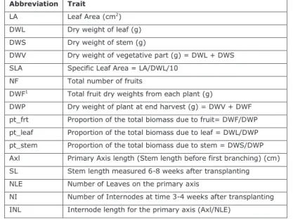
2.3.3. Trait evaluation
In this study, we analysed 9 physiological traits representing vegetative and generative development of pepper plants and 7 derived traits, being functions of the original traits (Table 2.1). The vegetative traits were measured via destructive harvesting at the end of the trials. The vegetative traits recorded include leaf area (LA), dry weights of leaves (DWL), stem
(DWS) and vegetative plant parts (DWV=DWL+DWS), specific leaf area (SLA=LA/DWL), the primary axis length (Axl) given as length of primary axis from cotyledons to first branching, number of leaves on primary axis (NLE), mean internode length of primary axis (INL=Axl/NLE). Other vegetative traits included stem length (SL) and number of internodes (NI) measured 6-8 weeks after transplanting. Recorded fruit traits included total number of fruit (NF) and total fruit dry weight (DWF) given as the sum of dry weight of all the fruits harvested during the growing season and the fruits on the plant at the final destructive harvest. DWF was taken to represent yield. Also calculated were the total plant biomass (DWP=DWV+DWF) and the proportion of total biomass in the leaves (pt_leaf), stem (pt_stem) and fruits (pt_frt). For each environment, trait distributions, correlations and pattern of variation across genotypes and blocks were obtained by using statistical and visualization tools after removing outliers.
Table 3.1 Traits measured in each of the four SPICY environments (experiments). Abbreviation Trait
LA Leaf Area (cm2) DWL Dry weight of leaf (g) DWS Dry weight of stem (g)
DWV Dry weight of vegetative part (g) = DWL + DWS SLA Specific Leaf Area = LA/DWL/10
NF Total number of fruits
DWF1 Total fruit dry weights from each plant (g)
DWP Dry weight of plant at end harvest (g) = DWV + DWF pt_frt Proportion of the total biomass due to fruit= DWF/DWP pt_leaf Proportion of the total biomass due to leaf = DWL/DWP pt_stem Proportion of the total biomass due to stem = DWS/DWP Axl Primary Axis length (Stem length before first branching) (cm) SL Stem length measured 6-8 weeks after transplanting NLE Number of Leaves on the primary axis
NI Number of Internodes at time 3-4 weeks after transplanting INL Internode length for the primary axis (Axl/NLE)
1representative for yield
2.3.4. Phenotypic analysis
The traits in each environment were univariately analyzed using linear mixed models. We
adopted a model specification as proposed in Piepho et al. (2006) to analyse the data on all
the RILs including the parents and F1. The linear mixed model used was of the form:
= + + ( ) + ( ) + + ( ∗ ) + , (2.1)
where Y represented a phenotypic trait value, μ was the overall mean, B, R(B) and C(B)
represented block, row-within-block and column-within-block effects respectively. M was a
4-level factor used to obtain and test phenotypic mean differences among the parents (YW,
CM 334), F1 and RILs. G stood for all the 152 genotypes. We introduced a variable (Z), coded
0 for parents and F1; and 1 for RILs. This allowed us to handle parents and F1 as fixed and the
149 RILs as random. Now the random RIL effect was modeled as Z*G. This induced a genetic variance of zero for the parents and a common genetic variance for the RILs. Z was
declared as quantitative in our SAS model statements. Defining Z as quantitative ensured that
no genetic effects were induced for the parents (Piepho et al., 2006). All other non-genetic
effects were captured in ε term.
In the NL environments, block was assumed random for recovery of inter-block information
since not all RILs were present in all the blocks (unbalanced). The variance components for
the random effects were estimated using restricted maximum likelihood (REML) (Littell et
al., 2006). Since RILs were assumed random, they were estimated using best linear unbiased
prediction (BLUP) as against the use of best linear unbiased estimation (BLUE) where RILs are treated as fixed. We however investigated the use of both for our data and found that both BLUE and BLUP results were very similar with correlation of about one, despite the
shrinkage factor in BLUP. These analyses were performed in SAS (Saxton, 2004; Littell et
al., 2006). Trait heritabilities were calculated using the measure based on BLUP as proposed
by Cullis et al. (2006).
= 1 − , (2.2)
where σg2 was the genotypic variance and vBLUP was the mean BLUP variance. The genetic correlations (ρg) between traits in each environment were estimated from the estimates of
variances and covariances obtained from a multivariate REML under the mixed model
procedure in SAS (Littell et al., 2006). The use of multivariate REML was preferred over
classical multivariate analysis of variance (MANOVA) as it can handle unbalanced data.
The dominance coefficient (k) for all traits was calculated from the expression: (1 + ) = ,
where was the overall additive effect in the CM334 parent = and d was the
mean difference between the F1 and YW (Lynch and Walsh, 1998). When -1<k<0, the YW
contribution was dominant over that of CM334 and when 0<k<1, CM334 was dominant. If k
< -1 or k > 1 and the phenotypic mean of the F1 exceeded that of the parent considered to
represent the desirable parent, we talk of heterosis. Transgressive segregation means that the phenotypic values of some of the RIL offspring were outside the range of parental phenotypic means. Transgressive segregation was declared substantial when the proportion of RILs with
phenotypes lower than the lower parent (denoted Qmin) - or higher than the higher parent
(denoted Qmax), was 50 percent or higher. We also compared phenotypic means of F1 and
RILs using expression DRIL. The statistic DRIL expressed difference in the means of RIL and
F1 (DRIL = RIL-F1) where RILs are phenotypically superior to F1 if DRIL > 0.
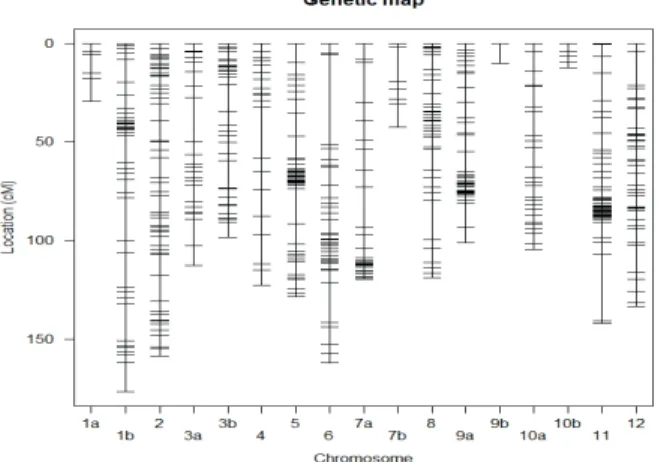
2.3.5. Marker data and Linkage map
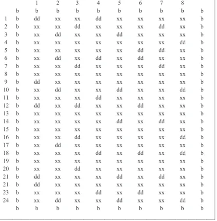
The first genetic linkage map (Figure 2.1) used the map similar to that of Barchi et al. (2007). A final set of 493 markers were assembled into 17 linkage groups (LG) covering 1775 cM. These were assigned to the 12 pepper chromosomes based on known positions of SSR markers. The list of publicly-owned markers used for the map construction is available as a supplementary material (Supplemental A1). Five chromosomes had two linkage groups that could not be joined due to insufficient linkage. The percentage of missing genotype information across the full set of markers was low (6.8%). The quality controls conducted
included checks on segregation distortion, recombination fraction and number of crossover events.
Figure 3.1 Initial Genetic linkage map used in the EU-SPICY experiments
2.3.6. QTL estimation
Many of the traits under investigation were assumed to be controlled by multiple QTLs which made a single QTL model inappropriate. We used a multiple-QTL mapping procedure
(MQM) (Jansen, 1993; Arends et al., 2010) for each trait in each environment.
= + ∑ + , (2.3)
where Y was the phenotypic response, μ the population mean, αq was the additive effect of
QTL q, xq was a marker-genotype indicator variables (0-1) and e was the residual term. The
package qtl (Broman and Sen, 2009; Arends et al., 2010) of the software R
(R-Development-Core-Team, 2011) was used to deploy the MQM approach in five steps. Firstly, the missing marker genotypes were imputed with their probabilities conditional on neighbouring marker information. Secondly, an initial single QTL scan equivalent to simple interval mapping was performed and a global significance threshold for QTL selection across all traits was determined via a permutation test of 1000 replicates. The obtained significance threshold was equal to a LOD score of 2.9. Thirdly, the MQM model was fitted by forward selection. Fourthly, a backward elimination strategy was applied to the full model with all earlier selected QTLs included to remove the non-significant QTLs and to arrive at the final QTL model. The QTL location confidence intervals were estimated from the final QTL using a Bayes credible interval with the assumption that there was one and only one QTL on the LG of interest for a given trait (Broman and Sen, 2009). This was mostly true for our data except for one trait (INL) on LG 1b in NL1. Lastly, the resulting final QTL model was evaluated to
obtain size and direction of QTL effects. Also, the QTL heritability HQ2 (proportion of
phenotypic variance due to a QTL) was estimated directly from the difference of the
log-likelihood (LOD) scores using the relationship: = 1 − 10 (Broman and Sen, 2009).
Pleiotropic QTLs were evaluated via visual inspection of the estimated QTL positions for different traits: QTLs with overlapping confidence intervals were declared to be the same QTL, i.e., a QTL with pleiotropic effects.
2.4.
Results
2.4.1. Traits evaluation
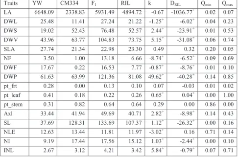
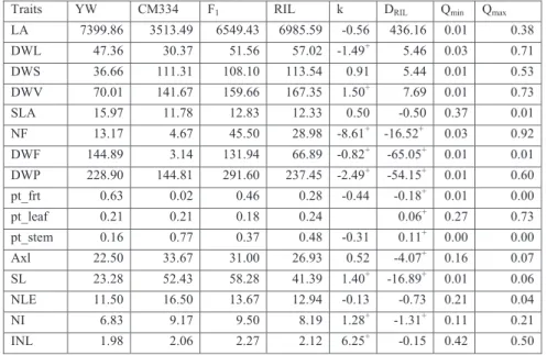
The phenotypic means for the parents, F1 and RILs for the SP2 environment (as an
appropriate representative) are presented in Table 2.2 and the means pertaining to the other environments are given in Appendix 2A. The parental means were clearly different for most of the traits. CM334 showed longer stem and internode lengths (Axl, SL and INL), heavier stem and total vegetative dry weight (DWS & DWV) and higher number of internodes (NLE and NI). In contrast, YW had higher values for fruit and leaf related traits. This parent showed bigger and heavier fruits, higher partitioning into fruit (pt_frt), higher leaf area (LA) and leaf dry weight (DWL). These results were consistent with previously reported results for these
pepper cultivars (Barchi et al., 2009). These contrasts between parental values were consistent
across the environments. For many traits, the F1 had higher mean values than the averaged
parental means especially for vegetative traits (e.g. DWL, DWS, DWV, DWP, Axl, SL and INL). The RILs showed substantial transgressive segregation for some traits (e.g. DWS, DWV, NF and DWP), where the transgression was in the direction of the parent with higher phenotypic values.
Table 3.2 Phenotypic Mean comparison for environment SP2
Traits YW CM334 F1 RIL k DRIL Qmin Qmax LA 8198.46 5985.77 10372.52 9980.89 -2.97+ -391.63 0.04 0.73 DWL 36.25 32.95 46.23 52.26 -7.05+ 6.03 0.04 0.91 DWS 29.02 87.28 88.44 95.55 1.04 7.11 0.00 0.62 DWV 72.27 120.22 134.68 147.62 1.60+ 12.94 0.01 0.80 SLA 22.85 18.34 22.60 19.25 -0.89 -3.35+ 0.34 0.05 NF 10.83 23.00 40.17 37.41 3.82+ -2.76+ 0.01 0.90 DWF 104.62 12.51 89.27 87.13 -0.67+ -2.14 0.01 0.31 DWP 176.90 132.73 223.94 234.94 -3.13+ 11.00 0.01 0.90 pt_frt 0.58 0.10 0.40 0.36 -0.25 -0.04 0.01 0.00 pt_leaf 0.25 0.25 0.21 0.23 0.02 0.80 0.20 pt_stem 0.16 0.66 0.39 0.41 -0.08 0.02 0.00 0.01 Axl 20.83 28.83 34.00 25.28 2.29+ -8.72+ 0.17 0.22 SL 23.83 76.33 83.33 67.38 1.27+ -15.95+ 0.00 0.27 NLE 9.33 13.50 11.33 9.87 -0.04 -1.46+ 0.44 0.01 NI 8.50 11.67 10.83 10.12 0.47 -0.71 0.09 0.08 INL 2.23 2.15 3.01 2.60 -20.5+ -0.41+ 0.14 0.79 k = Dominance coefficient
DRIL = Difference in the means of RIL and F1
Qmin = Proportion of RILs with phenotypes lower than the lower parent
Qmax = proportion of RILs with phenotypes higher than the higher parent +Significant at 0.05 level of significance
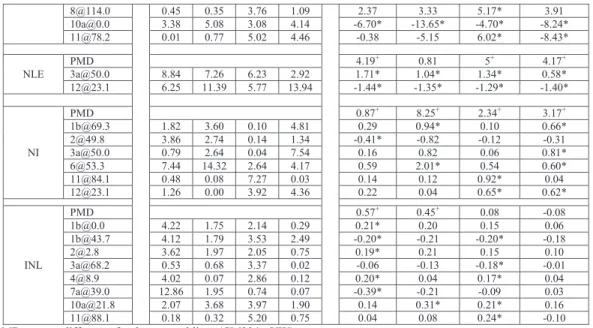
In the SP2 environment (Table 2.2) the YW contribution was dominant over CM334 (-1<k<0) for SLA, DWF, pt_frt, pt_stem and NLE while the CM334 contribution was dominant for NI (0<k<1). Heterosis in the direction of YW (k < -1) was observed for LA, DWL, DWP and INL while heterosis in the direction of CM334 (k > 1) was observed for DWS, DWV, NF, Axl and SL. The result for NF in SP2 is different from other environments in that the dominance for NF was derived from YW in all the other environments except SP2. Many
traits that showed heterosis also displayed substantial transgressive segregation and often in the same direction (Table 2.3). In all the environments, SLA and NLE for example showed
consistently higher value of Qmin than Qmax. Pt_leaf also showed higher Qmin than Qmax in NL2
and SP2.While LA, DWL, DWS, DWV, DWP and NF showed higher Qmax in all
environments. For some of the traits (e.g. NF, DWF, Axl and SL) RILs were phenotypically
inferior to F1 as F1 displayed higher phenotypic values consistently in the four environments.
For other traits, the sign of DRIL varied across environments. As examples, for LA a positive
DRIL was only found in SP1 and DRIL was positive in the SP environments for DWL, DWS,
DWV and negative in NL environments.
Table 3.3 Traits showing heterosis and substantial transgressive segregation Heterosis Transgressive segregation NL1 NL2 SP1 SP2 NL1 NL2 SP1 SP2 LA Y- T2 DWL Y- Y- Y- Y- T2 T2 DWS Y+ Y+ Y+ T2 T2 T2 T2 DWV Y+ Y+ Y+ Y+ T2 T2 T2 T2 SLA Y+ T1 NF Y- Y- Y- Y+ T2 T2 T2 T2 DWF DWP Y- Y+ Y- Y- T2 T2 T2 T2 pt_frt pt_leaf T1 T2 T1 pt_stem T2 Axl Y+ Y+ SL Y+ Y+ Y+ Y+ NLE Y- T1 NI Y+ Y+ Y+ T2 INL Y+ Y+ Y+ Y- T2 T2 T2
Y- = presence of heterosis in the direction of YW; Y+ = presence of heterosis in the direction of CM334; T1 = presence of substantial transgression in the direction of parent with lower phenotypic mean (i.e. high Qmin) and
T2 = presence of substantial transgression in the direction of parent with higher phenotypic mean (i.e. high Qmax).
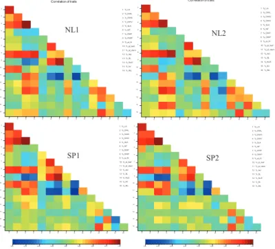
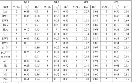
2.4.2. Heritability & genetic correlation
The heritability estimates (HT2) of traits were consistently high across the environments with
average of 0.86 and varied from 0.43 – 0.96 (Table 2.4). HT2 were mostly higher in the SP
environments than in the NL environments. Genetic correlations as a measure of association between traits within each environment were calculated. The correlations were found to show similar patterns across the environments (Figure 2.2). Fruit-related traits (DWF, NF and pt_frt) were positively correlated. Vegetative-related traits (LA, DWL, DWS, and DWV) were also positively co