Physically-based Simulation of Tornadoes

(1)

by

Xiangyang Ding

A thesis

presented to the University of Waterloo in fulfilment of the

thesis requirement for the degree of Master of Mathematics

in

Computer Science

Waterloo, Ontario, Canada, 2004 c

(2)

I hereby declare that I am the sole author of this thesis. This is a true copy of the thesis, including any required final revisions, as accepted by my examiners.

I understand that my thesis may be made electronically available to the public.

(3)

In this physically-based tornado simulation, the tornado-scale approach techniques are applied to simulate the tornado formation environment. The three-dimensional Navier-Stokes equations for incompressible viscous fluid flows are used to model the tornado dy-namics. The boundary conditions applied in this simulation lead to rotating and uplifting flow movement as found in real tornadoes and tornado research literatures. Moreover, a particle system is incorporated with the model equation solutions to model the irregular tornado shapes. Also, together with appropriate boundary conditions, varied particle con-trol schemes produce tornadoes with different shapes. Furthermore, a modified metaball scheme is used to smooth the density distribution. Texture mapping, antialising, anima-tion and volume rendering are applied to produce realistic visual results. The rendering algorithm is implemented in OpenGL.

(4)

Acknowledgements

The time as a graduate student at the University of Waterloo has been the best period of my life since I came to Canada, and for that wonderful experience I owe many thanks. I had one excellent advisor, Dr. Justin Wan. I became to be interested in scientific computing after I took Dr. Wan’s CS370 class - “Introduction to Scientific Computa-tion.” His teaching and advices at that time inspired me choosing this tornado simulation topic which is both interesting and challenging. Dr. Wan have had a profound influence on every process of this project. His guidance and supervision keep my research on the right direction and help me find out the appropriate solutions in modeling, rendering and animation. He also treated me as an equal researcher who is just less experienced and needs to be taught about problem-solving techniques. Dr. Wan also gave me freedom in implementation, choosing OpenGL in the rendering and parameter selection in anima-tion. In addition, he encouraged me to think creatively to find out the most appropriate boundary conditions and improve the visual effect. Dr. Wan’s advices are critical to my studies, academic writing and the success of this simulation project. Thanks for all of these, Justin!

I took the course CS888 – “Simulation of Natural Phenomena” from Dr. Gladimir Baranoski. The knowledge I learned from him, such as the simulation constraints and trade-offs, is very important to the success of this project. His experience in natural phenomena simulation, especially aurora simulation, is invaluable for me to choose the best parameters in rendering and animation. Also Dr. Baranoski’s stamina in aurora simulation encouraged me to work hard and always made me confident. Moreover, I

(5)

the density calculation and rendering steps in this tornado simulation. In addition, Dr. Baranoski’s support on my Curupira account was very helpful. Finally, thanks for the nickname – “Mr. Tornado,” I like it very much.

I would like to thank Dr. Bruce Simpson for his interests in this project and agreeing to read this thesis. My simulation knowledge and mesh generation techniques learned from him in CS476 and CS870 improve my background in scientific computing and are very helpful to this simulation project. Moreover, I thank him for his humour and patience in our talks and meetings.

I thank my family, especially my parents and my wife - Chunhui, for their encourage-ment and support. Thanks for Chunhui’s comencourage-ments on the simulated features. I owe her a lot of time to be together.

Finally, I thank all the friends in Scientific Computing group for their interests in this project, especially Shannon for his help on Latex and Amelie for her technical support on my machine - Scicom8.

(6)

List of Tables

2.1 The Fujita Scales with intensity and wind speed (Redrawn from Glossary of Meteorology [16]) . . . 13

3.1 The comparisons on modeling and boundary conditions between Trapp et al.’s simulation [38] and this simulation . . . 32

(9)

2.1 The projections of vortex streamlines onto: (a) the vertical plane through the axis of the vortex, (b) the horizontal plane. (Redrawn from [21]). . . . 12 2.2 (a) A tornado with a funnel shape on the plains of North Dakota, USA.

(http://ww2010.atmos.uiuc.edu/(Gh)/guides/mtr/svr/torn/home.rxml) (Cour-tesy of National Severe Storms Laboratory (NSSL), USA). (b) A tornado in USA with an unusual shape making a right-angle bend in the mid-dle. (http://www.weatherstock.com/tornadocat3.html) (Courtesy of the Weatherstock, USA). . . 15

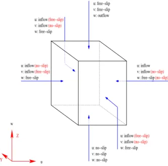
3.1 Coordinate environment and boundary conditions of the model applied in this tornado simulation. The boundary conditions inside the parentheses are used in Trapp et al.’s [38] simulation. . . 23 3.2 Velocity directions onX-Y plane to simulate the counter-clockwise rotation

(10)

LIST OF FIGURES

3.3 A better approach to assign velocity directions onX-Y plane for simulating the counter-clockwise rotation in the Northern hemisphere. The combined velocity direction changes continuously. . . 28 3.4 The vertical shear flow profile applied on the boundary. (a) Applied only on

the right boundary in Trapp et al.’s simulation [38] to produce horizontal rotation. (b) Applied on all 4 vertical boundaries in this simulation to generate interesting tornado shape in addition to the horizontal rotation. . 30 3.5 The magitude exponential distribution of w on the top boundary. . . 31 3.6 Staggered grid applied in 2D and 3D. (a) In 2D, velocities (u, v) and

pres-sure (p) are in different locations on the plane. (Redrawn from Griebel et al. [17]). (b) In 3D, velocities (u, v, w) shift by half a cell length along the positive X, Y and Z coordinate directions and they locate at the cell boundary plane centers while pressure (p) is at the cell center. . . 33 3.7 Staggered arrangement of the unknowns on a 2D domain after an extra

boundary strip of grid cells is introduced (Redrawn from [17]). . . 34

4.1 The decomposition of velocity and centrifugal force for a particular particle in the bottom debris swirling simulation. (a) Velocity decomposition. (b) Centrifugal force decomposition. . . 45 4.2 A diagram to show how a 2D dataset is modified after a metaball scheme

with radius 3 is applied. The density on each grid point is computed based on the density calculation function applied in this tornado simulation. . . . 51

(11)

4.3 The mesh diagrams of an original dataset and the smoothed dataset after metaball schemes are applied: (a) is the density distribution of the data presented in Figure 4.2(a) while (b), (c) and (d) are the density plots after metaball smoothing with metaball size 1, 2 and 3, respectively. The density on each grid point is computed based on the density calculation function applied in this tornado simulation. . . 52 4.4 The volume rendering algorithm used in Dobashi et al.’s cloud simulation

[7] is applied in this tornado simulation. Viewed from the viewer’s position, the image is generated based on the forward mapping (or splatting) method. 54

5.1 Velocity vectors on horizontal and vertical planes in the cube domain. (a) Velocity vectors of u and v close to the bottom boundary, on the middle and top X-Y planes. The counter-clockwise rotations are simulated and the rotation is more convergent to the plane center from the top to the bottom. (b) Velocity vectors of u, v and w on theX-Z plane sliced in the middle. . . 58 5.2 Simulated tornado shapes. (a) A funnel-shape tornado. (b) A tornado with

an angle. . . 60 5.3 Shape comparison with a real tornado. (a) A funnel-shape tornado in

Neal, Kansas, USA on May 30, 1982 (http://www.chaseday.com/tornado-neal.htm) (Courtesy of G. Moore). (b) A simulated tornado. . . 61

(12)

LIST OF FIGURES

5.4 Bottom debris swirling simulation and shape comparison with a real tor-nado. (a) An arrow-shape tornado with debris swirling effect at the bot-tom touched down near the town of Woonsocket, USA on June 24, 2003

(http://magma.nationalgeographic.com/ngm/0404/feature1/zoom3.html) (Cour-tesy of National Geographic). (b) A simulated tornado in an arrow shape

with debris swirling effect at the bottom. The simulated debris movement after centrifugal force and gravity applied can be observed in the corre-sponding animation. . . 62 5.5 Frames of an animation to show the dynamic change of tornado shape. . . 63 5.6 Frames of a real tornado animation which dynamically changes shape

dur-ing its lifetime (http://iwin.nws.noaa.gov/iwin/videos/tv5.avi) (Courtesy of the National Weather Service (NWS) of National Oceanic and Atmo-spheric Administration (NOAA), USA). . . 63

(13)

Introduction

As one of the severe phenomena in the world, “A tornado (from the Latin tornare, ‘to turn’) is the most violent storm nature produces” [13]. Tornadoes cause incredible amounts of damage and significant numbers of fatalities every year, thus making this phenomenon a major research topic. In this thesis, a physically-based tornado simulation is presented to produce tornadoes with interesting shapes and colors. Moreover, another research focus in this tornado simulation is to study tornado formation environment,

i.e., how boundary conditions are related to tornado shape evolution. The simulation is the combination of the numerical simulation and graphics rendering. The numerical simulation step is to simulate the general tornado flow movement, i.e., rotating on the horizontal planes and uplifting on the vertical planes. A particle system is introduced to define tornado volume and a volume rendering algorithm is used to visualize the flow movement based on the particle density.

(14)

1.1. MOTIVATION

1.1 will introduce the motivation of applying numerical simulation and graphics in this tornado simulation, Section 1.2 will talk about the general framework applied, and Section 1.3 will discuss the outline of this thesis.

1.1

Motivation

1.1.1

Why is numerical simulation used in this thesis

Before I discuss the reasons to apply numerical simulation in this thesis, I give a brief discussion about other tornado study methods, including their advantages and drawbacks. The first method to be introduced is tornado-chasing. Tornado-chasing has become an important activity for many scientists and weather enthusiasts to observe the tornado dynamics and collect the real data. The tornado videos recorded by tornado chasers offer us further understandings about its appearance and formation. Unfortunately, due to the difficulties to put the data recording equipments into the tornado path, the real data collection for tornado’s internal dynamics study is still not much successful today [4]. Instead of chasing tornadoes, on the other hand, satellite and radar images are also used to understand the flow dynamics of tornadoes [4]. But the cost is high in order to build enough satellites and radars to monitor tornadoes. Moreover, some researchers create their own “twisters” in laboratories [26] to study tornadoes. Tornadoes with different rotation speeds can be simulated by varying the apparatus condition, such as fan speed. The experiments conducted on the man-made tornadoes help scientists study tornadoes and understand their nature, for instance the destructive force and the formation process.

(15)

But this method is also cost expensive due to the fact that the simulation apparatuses need to be built or rebuilt.

In addition to the field and laboratory observations [4, 5, 8, 9, 13, 26, 31], mathematical modeling [19, 22, 27, 30, 34] and numerical simulation [12, 23, 28, 33, 36, 38] have been developed for various aspects of tornado studying. For example, applied originally in the simulation of other phenomena, such as turbulence [27, 28], cloud [23] and fluid flow [34, 38], varied models are researched to study tornado’s physical properties. Some models [30] are in cylindrical coordinates (2D) and assume that tornadoes are in axisymmetric internal structure while some others [38] are in the cube domain (3D) with the emphasis on asymmetric flow study. At the same time, different numerical methods, such as finite difference method and finite volume method, are applied to solve the model equations. Such modeling and simulation research lead to better understandings of tornado flow structures.

Although numerical simulation1 _{has some disadvantages, such as the difficulties to}

find the accurate model to represent the simulated phenomena, but compared with other tornado research methods discussed earlier, numerical simulation has several apparent advantages. First, numerical simulation has no risks. What the researcher needs to do is to write computer programs to form and solve the mathematical equations instead of going to the field to chase tornadoes as a tornado chasing team does. Second, numerical simulation has lower money expenditure. For example, generally speaking, a computer with high computing performance is enough for numerical simulation; but in order to use satellite and radar images for tornado research, more money needs to be spent in building

(16)

1.1. MOTIVATION

satellites and radars, especially more than one satellites or radars are usually needed. The cost problem is the same in laboratory experiments where simulation apparatuses need to be built, and even rebuilt when a different tornado formation environment is simulated. Third, the tornado formation environment is easily to be studied in numerical simulation. For instance, we can test the model and research the tornado formation environment by applying varied boundary conditions in the simulation. The user just needs to modify the code of the computer programs without worrying about the replacement of the machine parts which maybe happen in laboratory experiments. Finally, numerical simulation can be done within a short period of time, such as several months or one year, but to build satellites, radars and laboratory equipments would be more time expensive. All these advantages make numerical simulation an important research approach in tornado studies.

In addition, compared with other tornado study methods, to use numerical simulation techniques for my tornado flow research is the reasonable choice because of the time limit and cost limitation in my graduate study. The numerical solutions of the physical model is used to produce the general flow movement observed in real tornadoes, i.e., rotating and uplifting. It is assumed that realistic flow modeling can lead to realistic tornado flow movement in the final rendered images.

1.1.2

Why is graphics applied

As discussed in the previous section, numerical simulation is one important research method in tornado studies. But the numerical simulation results in tornado research

(17)

literature focused mainly on the velocity, pressure and temperature fields without a sim-ulated realistic tornado image to show its movement, shape and color, thus making the simulation less visually interesting. So in this thesis, in addition to the simulated tor-nado flow, tortor-nadoes with interesting shapes and colors are also produced for realistic visual results. To do this, graphics techniques are employed to visualize the tornado flow generated in the numerical simulation step.

It needs to be noted that the graphics is combined with physically-based modeling in this thesis, but it is not in this case in the tornado studies. For example, created by using pure computer graphics techniques in entertainment field, visually appealing tornado images are widely used on TV programs and films, such as TWISTER [10], but their purposes are for entertainment only without taking into account the tornado physical dynamics.

We can see that the two approaches in natural phenomena simulation, numerical simu-lation and graphics, emphasize either physics or visual results, same as their applications in tornado simulation. As pointed out by Barr et al. [2] below, the ideal approach in natural phenomena simulation is to combine both of them:

These two approaches have begun to reach the limits of their ability without each other. The realism required in entertainment animation is beyond that obtainable without physically realistic models. Similarly, numerical simula-tions in the physical sciences are complex to the point of being incomprehen-sible without visual representations.

(18)

ad-1.2. PREVIEW

vantages of both numerical simulation and graphics rendering to avoid the either “pure simulation” or “pure animation” problem discussed in [2]. The numerical simulation tech-niques produce tornado flow simulation results from the physically modeling, and graphics rendering is used to visualize the flow movement. As the result of the combination, the user can see the simulated tornado flow rotating and going up. Also, with the application of animation, we can understand the tornado flow movement further. To the best of my knowledge, the combination of numerical simulation and graphics rendering has never been done in tornado studies. My intention is to provide some understandings about tornado flow generation and visualization to tornado researchers. I would be very happy if my work could contribute to the tornado research at some extent.

1.2

Preview

In this physically-based tornado simulation, the tornado-scale approach techniques [30] are applied to simulate the tornado producing environment. This approach has been widely used in laboratory experiments [6, 24, 33, 41] and numerical simulations [12, 27, 30, 36, 38] for tornado studies. The three-dimensional Navier-Stokes equations for incompressible viscous fluid flows are used in this thesis to model the tornado dynamics. The boundary conditions applied in this simulation lead to rotating and uplifting flow movement as found in real tornadoes and tornado research literatures.

To model the irregular tornado shapes, a particle system is incorporated with the model equation solutions. As will be discussed later in Section 4.1.2, to control the number and initial positions of particles generated at each time step is rather difficult due

(19)

to the following facts. First, the number of particles will influence the particle density in the domain, then the transparency and the final rendered image, so a good control scheme on the number of particles generated will give nice color variation effect as seen in real tornadoes. Second, the particle position attribute can change the shape of visualization results. For example, if the flow movements at certain places in the domain are part of tornado shape evolution process, but there are no or not enough particles at those locations, then some parts of the tornado shape will be missing in the final tornado images. As presented in Figure 5.2(a) and (b) in Section 5.2, with the same boundary conditions, different control schemes on the number of particles generated at each step produce tornadoes with different shapes. Moreover, gravity and centrifugal force are applied to some particles in this simulation to simulate the bottom debris swirling effect. In the bottom debris swirling simulation, to produce different particle motion paths from what other particles follow is also very challenging. Therefore, significant amount of time is spent on the parameter selection in the particle system in order to produce the realistic results.

In addition, a modified metaball scheme is applied in particle density calculation to smooth the density distribution. The metaball radius and interpolation functions used in this simulation lead to a continuous density distribution with the efficient computing speed at the same time. Furthermore, the density level discretization strategy applied subdivides the densities into certain levels with the time efficiency consideration as well. As a result, the density differences between levels are retained for color variation purpose in the rendering step.

(20)

1.3. OUTLINE

graphics techniques, such as texture mapping, antialising and animation, are applied for better visual results. Moreover, the blending factors used in OpenGL implementation achieve good blending effects in the combination of the object color with that of the background.

As the results demonstrated in Section 5.2, because the axisymmetric tornado struc-ture is not assumed in the modeling, tornadoes with different shapes are produced. The comparison between a simulated tornado and a real tornado shows that the model and boundary conditions applied in this simulation can generate a tornado with a similar shape as a real tornado has. Moreover, gravity and centrifugal force are applied to sim-ulate the bottom debris swirling effect. The simsim-ulated debris movement is qualitatively compared with a real tornado. Furthermore, the simulated dynamic shape change effect in a tornado presented in Figure 5.4 is also consistent with the shape change observation in a real tornado video.

1.3

Outline

In the following chapters, this tornado simulation will be discussed in details. First, Chap-ter 2 gives a brief overview about tornado phenomenon, especially its physical characChap-teris- characteris-tics closely related to this simulation. The comparisons of tornadoes with hurricanes and typhoons are also discussed, as well as the difficulties of tornado studies. Then in Chapter 3, the details of modeling and simulation are presented. It starts with the literature re-view and the introduction of simulation approaches generally used in tornado simulation. Then the model and the boundary conditions applied in this simulation are discussed, as

(21)

well as the numerical techniques used to solve the equations. Next, the particle system is introduced in Chapter 4. The metaball scheme and rendering algorithm are also covered. After that, validation will be discussed in Chapter 5, as well as the presentation of the simulation results. The comparisons between the simulations and real tornadoes will also be presented. Finally, this physically-based tornado simulation will be summarized in Chapter 6, and the limitations and future work will be discussed.

(22)

Chapter 2

Tornado Phenomenon

The introduction of tornado phenomenon is presented in this chapter. Firstly, I discuss the characteristics of a tornado in Section 2.1, as well as the comparisons of a tornado with other two closely related phenomena - hurricane and typhoon. Secondly, in Section 2.2, the difficulties of tornado research are discussed.

2.1

Tornado Characteristics

Before the introduction of tornado phenomenon, a brief overview about other two violent storms in the nature, hurricane and typhoon, will be given. These two phenomena have many similarities with tornadoes, such as the rotation and violence. But the most im-portant reason to discuss them is that the tornado formation process is closely related to hurricane and typhoon. For example, many tornadoes are actually spawned by hurricanes or typhoons [21].

(23)

In the Glossary of Meteorology [16], hurricane, typhoon and tornado are all clas-sified under the same term - “cyclone”. Cyclone is defined as “a large-scale circulation of winds around a central region of low atmospheric pressure, counter-clockwise in the northern hemisphere and clockwise in the southern hemisphere” [44]. One kind of cy-clone is the tropical cycy-clone which “originates over” the tropical oceans [16]. The terms “hurricane” and “typhoon” areregionallyspecific names for a strong tropical cyclone [20]. To be specific, hurricane is defined as a tropical cyclone with wind speed in excess of 32

m/s(70mph) in the Western hemisphere (North Atlantic Ocean, Caribbean Sea, Gulf of Mexico, and in the Eastern and central North Pacific) [16]. And typhoon is an identical phenomenon as a hurricane but it occurs in the Eastern hemisphere [16, 21]. From their definitions, we can see that hurricane and typhoon are regional phenomena which are very different from a tornado. Tornado is defined as an “violently rotating column of air, in contact with the ground, either pendant from a cumuliform1 _{cloud or underneath a}

cumuliform cloud” [16]. The wind rotation speed can be as low as 18 m/s (40mph) to as high as 135 m/s (300 mph), and the forward motion speed of a tornado averages around 40 mph [13], but can be as high as 68 mph. In addition to the strong vortical motion in a tornado, the “up-rushing currents of lifting strength” [13, 35] is also an important characteristic of it. The typical tornado flow structure is described in [28] as “the flow spirals radially inward into the center of the vortex that is basically a swirling and rising jet”. A schematic of such vortical and uplifting flows is shown in Figure 2.1.

As tornado is clearly defined as contacting with the ground [16], they are primarily

1

Generally descriptive of all clouds, the principal characteristic of which is vertical development in the form of rising mounds, domes, or towers [16].

(24)

2.1. TORNADO CHARACTERISTICS

(a)

(b)

Figure 2.1: The projections of vortex streamlines onto: (a) the vertical plane through the axis of the vortex, (b) the horizontal plane. (Redrawn from [21]).

an “over-land phenomena” while on the other hand, hurricane and typhoon are purely an “oceanic phenomena” because they finally disappear on the land where the “mois-ture source” does not exist [31]. Moreover, like hurricanes and typhoons, tornadoes are primarily in the summer, but in theory, tornadoes can occur at any time of the day throughout the year. Furthermore, tornadoes can happen on all continents and are only minutes long while hurricanes and typhoons can only happen in some specific regions and can last for days [16]. As a global phenomenon, tornadoes have been reported in many countries in the world, such as Canada, England, France, Holland, Germany, Hungary, Italy, Australia, India, Russia, China, Japan, even Bermuda Islands and Fiji Islands [13]. However, they are most frequent in spring and summer during the late afternoon on the central plains and in the Southeastern states in the United States [13, 16, 36]. Each year an average of a thousand tornadoes are reported in the United States [36]. In Canada, tornadoes are more frequently seen in the Southern provinces and Southwestern Ontario [9]. On average, about 60 tornadoes are reported each year in Canada.

(25)

Table 2.1: The Fujita Scales with intensity and wind speed (Redrawn from Glossary of Meteorology [16])

F-Scale Number Intensity Phrase Wind Rotaion Speed

F0 Gale Tornado 40-72 mph F1 Moderate Tornado 73-112 mph F2 Significant Tornado 113-157 mph F3 Severe Tornado 158-206 mph F4 Devastating Tornado 207-260 mph F5 Incredible Tornado 261-318 mph F6 Inconceivable Tornado 319-379 mph

Compared with other storms in the nature, a tornado is the most violent one [8, 26]. It is estimated that tornadoes cause about one billion dollars of damage per year in the United States. The destructive rotation in a tornado is the main cause for such violence and damage. Theodore Fujita and Alan Pearson [25] first linked the tornado rotation speed with the amount of damage it produced in 1971. The system they devised, called Fujita-Pearson scale, is widely used as a standard system to classify the intensity of a tornado. As shown in Table 2.1, this system rates tornadoes by 7 classes. Tornadoes with intensity scale F0 - F1 are weak, F2 - F3 are strong, and above F4 are violent. In Canada, no F5 tornadoes have ever been recorded, but a number of F4 events have been [9].

Some important physical characteristics directly related to the simulation of tornado dynamics are summarized in the following categories:

• rotation: the rotation direction of a tornado is counter-clockwise in the Northern hemisphere and clockwise in the Southern hemisphere [13]. The simulation results in Section 5.2 show that the counter-clockwise rotation in the Northern hemisphere

(26)

2.1. TORNADO CHARACTERISTICS

can be successfully produced by using the model and specific boundary conditions applied in this simulation. With the corresponding changes on the boundary con-ditions, the model used can be easily applied in the simulation of the clockwise rotation in the Southern hemisphere.

• shape: a tornado generally takes the shape of a cone or a cylinder or of a funnel in which tornado is equal or greater in diameter at the top than at the bottom [13]. But a tornado with funnel shape is the most common one [13]; see Figure 2.2(a) for an example of funnel-shape tornadoes. Such funnel shape is the result of the “rotary motion of extremely high speed” [5]. Tornadoes, however, can have some other shapes as well. For example, a tornado can be greater at the bottom [4, 13, 37]. And a tornado can also look like a snake or rope [4, 47] and even makes a “right-angle bend” [13] as it nears the ground. Figure 2.2(b) shows an example of bended rope-like tornadoes. The animation frames demonstrated in Section 5.2 show the simulation results of a funnel-shape tornado and a bended tornado. Moreover, after centrifugal force and gravity are applied in the particle system, the bottom debris swirling effect can be simulated. As presented in Figure 5.4, the simulated arrow shape tornado is qualitively similar to a real tornado.

• color: Laycock [26] describes that a tornado is generally gray or dark. When we see a tornado, what we are really seeing is the water vapor inside the wind or the sucked objects by the swirling strength because the wind itself is invisible [26]. If there is only water vapor in the wind, the color will be gray [26]. But if some objects, such as dirt, leaves and bark, are drawn to the wind, the tornado will

(27)

(a) (b)

Figure 2.2: (a) A tornado with a funnel shape on the plains of North Dakota, USA. (http://ww2010.atmos.uiuc.edu/(Gh)/guides/mtr/svr/torn/home.rxml) (Courtesy of National Severe Storms Laboratory (NSSL), USA). (b) A tor-nado in USA with an unusual shape making a right-angle bend in the middle. (http://www.weatherstock.com/tornadocat3.html) (Courtesy of the Weatherstock, USA).

be dark [26]. It should be noted that not all tornadoes are visible, for example, when a tornado moves through “comparatively dry and clean air” it is invisible [13]. But the visible tornadoes are more interesting to viewers, so to produce a tornado with color is one of our goals in the simulation for the best realistic simulation results. The volume rendering algorithm used in this simulation produces visual response with interesting colors as the observed real tornadoes. As shown in Section 5.2, the rendering algorithm applied can produce gray color and darker tornadoes. Tornadoes with other colors can also be simulated by choosing different backgrounds and wind colors.

(28)

2.2. TORNADO RESEARCH DIFFICULTIES

2.2

Tornado Research Difficulties

The study on tornado formation and its dynamics is always a challenging topic. Scientific research tells us that tornadoes are from the energy released in a thunderstorm and they usually occur under some specific atmospheric conditions, such as great thermal instability, high humidity, and the convergence of warm, moist air at low levels with cooler, drier air aloft [25]. In general, scientists understand that tornadoes form when a “rotating thunderstorm updraft” and a “gyratory wind” meet at the same place [25]. But latest tornado research finds that tornadoes can also be produced by “non-rotating” thunderstorms [34]. However, the most violent and “long-lived” tornadoes are produced in a special kind of thunderstorm, supercell2_{, where the wind rotation is important [34].}

Moreover, some other phenomena often provide the conditions for tornado formation. For example, tropical cyclones, an oceanic phenomena, usually spawn tornadoes before they disappear on the land [25]. The physical process involved is that when the tropical cyclones reach the land, they start decaying, the winds at the top decay faster thus a “strong vertical wind shear”3 _{is formed which is essential for tornado development [31].}

But many other uncertain factors still exist about how a tornado is formed [9]. Also, the physical data in a tornado, which is necessary for tornado dynamics study, is difficult to be recorded [4]. This is because it is hard to put equipment on the right positions

2

“An often dangerous convective storm that consists primarily of a single, quasi-steady rotating up-draft, which persists for a period of time much longer than it takes an air parcel to rise from the base of the updraft to its summit. Most rotating updrafts are characterized by cyclonic vorticity. The supercell typically has a very organized internal structure that enables it to propagate continuously. It may exist for several hours and usually forms in an environment with strong vertical wind shear. Severe weather often accompanies supercells, which are capable of producing high winds, large hail, and strong, long-lived tornadoes” as stated in [16].

(29)

since tornadoes are only minutes long and they move with “unpredictable” paths [4]. The film TWISTER was based on the work National Severe Storms Laboratory (NSSL) did in the middle of 1980’s [4]. NSSL tried for several years to put the equipment, called TOTO

(TOtable Tornado Observatory)4, into the “coming” path of a tornado, but it was very difficult to succeed. Samaras and National Geogrhphic [39] tried the similiar approach to put the probes, metal disks that can measure a tornado’s wind speed, direction, barometric pressure, humidity, and temperature through the embedded sensors, into the path of the tornado funnel. However, only five such instruments have been “deployed” successfully into the tornado paths after more than a decade of attempts.

In addition to the field quantitative observations of tornado chasing teams [4, 46], other tornado research methods have also been used in the understanding of the internal structure and dynamics of tornadoes, such as the development of radars, satellites and laboratory experiments5_{, but the improvement in modeling and numerical simulations}

plays an active role and has made significant advances. The detailed discussion will be given in the next chapter.

4

This device used “hardened” sensors that had been used to measure wind shear and severe downslope winds. It was designed to be mounted in a pickup truck and deployed in 30 s or less. Wind speed, wind direction, temperature, static pressure, and corona were recorded [4].

5_{The purpose of the laboratory experiments is to create flows that, to the extent that it is possible,}

are geometrically and dynamically similar to natural flows, in order that meaningful observations and

physical measurements can be made [6]. The equipment is called Tornado Vortex Chamber (TVC) [6].

By changing the speed of fan, scientists can control the air swirling speed. The more interesting thing is, when smoke is fed into the swirling air, they can even see the air moving [26].

(30)

Chapter 3

Modeling and Numerical Simulation

The use of mathematical model and numerical simulation in this thesis is to model and simulate the tornado flow movement, and then provide physical data at some extent for graphics rendering in order to combine the physically-based modeling and graphics in this tornado simulation. The details of the physically modeling theory, boundary conditions applied and numerical implementation of this simulation are discussed in this chapter. In Section 3.1, the modeling theory of tornado simulation is introduced, as well as the models used by scientists and the model used in this thesis. Then the boundary conditions applied in this simulation are discussed in Section 3.2. Finally, Section 3.3 introduces the staggered grid, the implementation of boundary conditions and the steps to solve the model equations.

(31)

3.1

Model Overview

The modeling study on tornado research can generally be divided into two categories: thunderstorm-scale simulations and tornado-scale simulations [30]. As discussed in [23, 30], the former category is pioneered by Klemp and Wilhelmson who present a model orig-inally for cloud simulation known as KW model, and then this model is applied in tornado simulation to numerically simulate the formation and dynamics of the thunderstorms that are responsible for tornado formation. On the other hand, tornado-scale simulation, pio-neered by Rotunno [30, 33], assumes that a particular rotating environment caused by the “convergence” of rotating flow along boundaries leads to the tornado-like1 _{vortices, and}

the models applied in this approach are intended to provide the details of the wind field in the tornado and an understanding of the dynamics that lead to the flow rotation structure. Because the domain boundary and initial conditions are easy to control in the tornado-scale simulation, many laboratory researchers [6, 24, 33, 41] produce miniature tornadoes inside the laboratory by simulating the rotating apparatus environment instead of sim-ulating the thunderstorm formation. Also, many tornado scientists [12, 27, 30, 36, 38] apply the tornado-scale approach in their numerical simulations to generate tornado-like rotation and uplifting flow by simulating a rotating environment.

But the physical models and boundary conditions applied in their tornado-scale sim-ulations vary due to different considerations on the process of tornado formation. For example, most tornadoes take the funnel shape in the real life, thus a tornado flow struc-ture is generally believed to be axisymmetric [12, 27, 30, 36]. Such assumption leads to

1_{This term could apply to any vortex caused by the convergence of rotating fluid along boundaries}

(32)

3.1. MODEL OVERVIEW

the fact that most of the numerical models are in 2D Polar coordinate system as presented by Sinkevich et al. [36] and Fiedler [12]. They all assume the tornado funnel rotating about a vertical axis with a known constant angular frequency. The model of Sinkevich

et al. [36] involves the two-phase (liquid and gas) turbulent heat and mass transfer while

Fiedler [12] uses an incompressible Navier-Stokes equations model applied in a cylinder domain. It is an axisymmetric convection model with a defined thermodynamic speed limit (the rotation speed) in a closed domain [12]. Navier-Stokes equations are also ap-plied in Trapp et al.’s [38] simulation, but the model is applied in 3D cube domain and they assume that the flow is compressible. Their goal is to study how tornadoes, which appear “at least locally axisymmetric”, are born out of the asymmetric surrounding flow with initial horizontal velocity only [38]. As will be discussed in Section 3.2, their sim-ulation is by simulating a tornado-producing environment, but they do not simulate a rotating environment initially as other tornado-scale simulations generally do. In this tornado simulation, the tornado-scale simulation approach is applied.

The physical model used in the tornado-scale simulation here is the governing equa-tions of fluid mechanics – the Navier-Stokes equaequa-tions [17]. This model was originally de-veloped to simulate the viscous and unsteady fluid flow dynamics [3, 17, 40]. But recently, it has been widely used in computer graphics for the simulation of physical phenomena, such as water [14], smoke [11], cloud [18], fire [29] and the growth of plant leaf [40]. As described above, this model has also been applied in tornado simulations [12, 28, 30, 38]. In the modeling of this simulation, the equations employed are for incompressible fluid flow, which have also been considered in [12, 28, 30]. However, the axisymmetric tornado internal structure is not assumed here, thus this simulation allows the tornado to form

(33)

any shape. Moreover, this model is applied in 3D Cartesian coordinate system instead of the Polar system. The 3D cube model coordinate environment is depicted in Figure 3.1.

The standard Navier-Stokes equations applied in this simulation can be written in dimensionless form as:

ut+ (u· 5)u =

1

Re4u− 5p+g 5 ·u = 0,

whereuis the fluid velocity vector,pis the pressure,g denotes body forces such as gravity, and Re is the Reynolds number which represents the viscosity of the fluids [17, 40]. In our mathematical model, the motion of the liquid is described by the evolution of two dynamic field variables, velocity and pressure. In three dimensions, the velocity vector is composed of the vertical component walong Z and 2 other componentsu andv onX-Y

plane whereuis alongX andv is alongY. The 3D Navier-Stokes equations in component form can be given as:

(34)

3.1. MODEL OVERVIEW ∂u ∂t + ∂p ∂x = 1 Re µ ∂2_u ∂x2 + ∂2_u ∂y2 + ∂2_u ∂z2 ¶ −∂u 2 ∂x − ∂uv ∂y − ∂uw ∂z +gx ∂v ∂t + ∂p ∂y = 1 Re µ ∂2_v ∂x2 + ∂2_v ∂y2 + ∂2_v ∂z2 ¶ − ∂uv ∂x − ∂v2 ∂y − ∂vw ∂z +gy ∂w ∂t + ∂p ∂z = 1 Re µ ∂2_w ∂x2 + ∂2_w ∂y2 + ∂2_w ∂z2 ¶ − ∂uw_∂x −∂vw_∂y −∂w 2 ∂z +gz continuity equation: ∂u ∂x + ∂v ∂y + ∂w ∂z = 0, where

u: horizontal velocity of fluid flow (along the X coordinate). Positive direction is right.

v: horizontal velocity of fluid flow (along the Y coordinate). Positive direction is inward.

w: vertical velocity of fluid flow (along the Z coordinate). Positive direction is up.

gx, gy, gz: gravity component on X, Y and Z coordinates respectively.

Note that since the axisymmetric flow structure is not assumed in modeling, this model can be applied to simulate tornadoes with different shapes, as shown in Section 5.2.

(35)

w: free−slip w: free−slip u: inflow v: inflow v: inflow u: inflow u: no−slip v: no−slip w: no−slip u: free−slip v: free−slip w: outflow u Z X Y v w (no−slip) (no−slip) (no−slip) u: inflow v: inflow(no−slip) w: free−slip v: inflow u: inflow(no−slip) w: free−slip (free−slip) (free−slip) (free−slip)

Figure 3.1: Coordinate environment and boundary conditions of the model applied in this tornado simulation. The boundary conditions inside the parentheses are used in Trappet al.’s [38] simulation.

(36)

3.2. BOUNDARY CONDITIONS

3.2

Boundary Conditions

Before the boundary conditions applied in this simulation are presented, a short introduc-tion on the definiintroduc-tions of different boundary condiintroduc-tions is given first as discussed in [17]. The detailed explainations in mathematical form and how to implement these conditions in this simulation will be given in Section 3.3.

1. no-slip condition: the fluid is at rest there.

2. free-slip condition: no fluid penetrates the boundary. Contrary to the no-slip con-dition, however, there are no frictional losses on the boundary.

3. inflow condition: the value of the velocity component is given explicitly. The flow can go in or out of the boundary.

4. outflow condition: the velocity does not change in the direction normal to the boundary.

Note that as discussed in Section 3.3, the boundary conditions are applied to the individual velocity component, i.e., velocity u, v and w at the same boundary position can have different boundary conditions. This technique is applied in tornado-scale simulations, such as in [38].

Tornado studies reveal that the boundary conditions are essential in tornado-scale simulation to achieve the rotation and uplifting movement [30, 33]. The general approach applied in tornascale simulation is to force the flow rotating along the sides of the do-main boundaries and draw the flow out of the top dodo-main with some boundary conditions, such as outflow condition [30].

(37)

As introduced in Section 3.1, Trapp et al. [38] present a tornado-scale simulation on how a symmetric tornado is born out of the asymmetric surrounding flow. The boundary conditions applied in their simulation are illustrated in Figure 3.1. In their simulation, a fixed vertical shear flow enters the cubic domain through the right boundary plane in Figure 3.1, the vorticity associated with this shear flow is horizontal and “transverse” to the inflow velocity [21, 34, 38]. To simulate the uplifting flow effect, they use outflow condition for w and free-slip for u and v on the top boundary. The extraction flow distribution and how fast it is depend on how outflow condition is applied on w. For example, to simulate the flow exhaust effect that extraction is more violent around the center of the top boundary, they set the values of w on the top based on the exponential function in which the magitude is smaller closed to the edge and bigger approaching the top boundary center.

The boundary condition studies in this thesis is based on Trapp et al.’s. In their simulation, the outflow condition on the top is reasonable to simulate the fact, as discussed by Rotunno [34], that the low pressure on the top of tornado causes the air “upward” which finally generates the “updraft”. So in this simulation, the same boundary condition is applied on the top (See Figure 3.1). But the boundary conditions on the vertical planes are different from theirs. For instance, on the left boundary plane in Figure 3.1, the no-slip condition for u (along the X direction) used in Trapp et al.’s simulation assumes that there is no flow in and out of that plane, which in turn isolates tornado from the natural environment. In fact, it seems awkward to force the flow to go up or down on that plane. The problem is the same to v (along the Y direction) on the back and front boundary planes. In their discussion, they name these boundaries as “stagnation

(38)

3.2. BOUNDARY CONDITIONS

walls” [38]. Although such boundary condition set up is necessary to their simulation, different boundary conditions are applied in the simulation here in order to simulate a more reasonable tornado formation environment. To do this, inflow condition is used for bothu

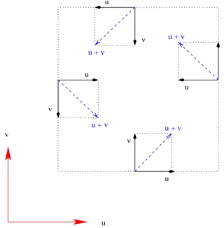
and v on theX-Y planes. It assumes that flow can go in or out of the vertical boundaries at a flow speed explicitly given. Moreover, this simulation is to simulate the rotating environment initially as a tornado-scale simulation generally does. Tornado research has shown that rotation can be generated by applying inflow condition on one boundary only [34, 38], but to obtain the rotation faster, inflow condition is applied on all 4 vertical boundaries (excluding top and bottom) in this thesis. In addition, u and v are assigned at specific directions along the vertical boundaries as shown in Figure 3.2. This rotation implementation is to simulate the counter-clockwise rotation as the tornadoes have in the Northern hemisphere. Note that one problem to this velocity direction assignment is that the direction of the combined velocity changes sharply at the corners. For example, in Figure 3.2, the combined velocity on the left boundary has ₋45◦ _{direction with respect}

to the positive direction of X axis. On the other hand, the direction is 45◦ _{on the bottom}

boundary. Such sharp direction change at the bottom left corner may cause flow eddy. So a better approach is to assign the flow velocities in continuous changing directions shown in Figure 3.3. But such approach would make the boundary condition implementation very complicated. So to simplify the implementation, the velocity directions are assigned based on Figure 3.2. And to be noted that the expected fluid eddy cannot be seen from the final tornado images presented in Section 5.2. One reason maybe that the flow eddy at the corner is too small compared with the flow in the middle of the domain.

(39)

u v u u v v u + v _{u + v} u + v u + v Y X u v v u

Figure 3.2: Velocity directions on X-Y plane to simulate the counter-clockwise rotation in the Northern hemisphere.

But how to appropriately implement such inflow conditions for u and v on those boundaries leads to more subtle questions. For example, what is the magnitude of u

or v at a certain vertical level? And how does the magnitude change along the vertical direction from the bottom to the top, e.g., increasing, decreasing or being a constant? Previous tornado studies [34, 38] show that applying a vertical shear flow with varied velocity magnitude on one of the vertical boundaries is a reasonable choice. For example, in Trappet al.’s [38] simulation, a vertical shear flow, as presented in Figure 3.4(a), enters the domain through the right boundary. Also as pointed out by Rotunno [34] and Houze [21], such vertical shear flow generally leads to the horizontal rotation at the end. At the early step of this simulation, such vertical shear flow approach is applied on one boundary,

(40)

3.2. BOUNDARY CONDITIONS Y X v u u + v u + v u + v u + v

Figure 3.3: A better approach to assign velocity directions onX-Y plane for simulating the counter-clockwise rotation in the Northern hemisphere. The combined velocity direction changes continuously.

(41)

and with the combination of the outflow condition on the top boundary, the tornado-like rotation and uplifting flow effect are simulated. In addition to these simulation results, note that the tornado studies in this simulation also want to produce simulated tornadoes with interesting shapes. The current tornado numerical simulation results are only lim-ited to the velocity, pressure and temperature fields without a simulated tornado image to show its movement, shape and color, thus making the simulation less interesting. But in this tornado simulation, research on how boundary conditions affect tornado shapes are conducted. To the best of my knowledge, research on how boundary condition leading to a final realistic tornado shape has never been found in tornado numerical simulation literature. Based on the specific boundary conditions applied on the vertical boundaries, the experiments conducted in this simulation show that only applying the vertical shear flow on one boundary can produce rotation, but it cannot generate a nice tornado shape at reasonable simulation time. On the other hand, as Figure 5.2(a) in Section 5.2 demon-strates, by applying shear flow on all 4 vertical boundaries with certain varied velocity magitudes can lead to interesting funnel shape within reasonable time. To simulate such funnel shape, on the 4 vertical boundaries, we can set the velocity magnitude of u and v

decreasing from the bottom to the top. Note that this idea focuses on how to generate the expected tornado flow and shape. Since I have not found tornado research literatures about how boundary conditions affect the tornado shapes, unfortunately I cannot refer to tornado scientists’ work to verify such magnitude assignment. In my simulation, one implementation of this magitude assignment is to setu andv equal to 2_×nz−k

nz , wherenz

is the number of segments in the numerical discretization along the Z direction, k is the index along the Z coordinate and it is from 0 to nz from the bottom to the top. As the

(42)

3.2. BOUNDARY CONDITIONS Z 0.5 0.0 1.0 1.0 u(Z) 0.5 1.0 0.0 Z 2.0 v(Z) u(Z),

(a)

(b)

Figure 3.4: The vertical shear flow profile applied on the boundary. (a) Applied only on the right boundary in Trapp et al.’s simulation [38] to produce horizontal rotation. (b) Applied on all 4 vertical boundaries in this simulation to generate interesting tornado shape in addition to the horizontal rotation.

velocity profile demonstrated in Figure 3.4(b), for u and v near the bottom, k is small, thus leading to larger magitudes of u and v. When u and v are close to the top, k is bigger, so u and v are smaller on the top boundary.

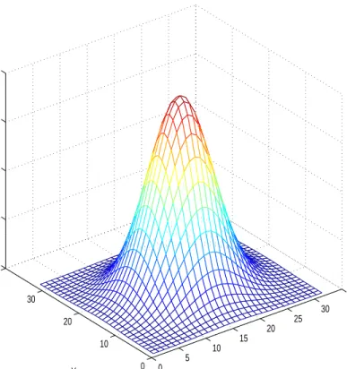
Moreover, the exponential function used to control the velocity magitude distribution of w on the top is same as Trapp et al.’s [38]:

wi,j,nz = 2e − ·µ i nx−0.5 r ¶2 + µ j ny−0.5 r ¶2¸ , (3.1)

(43)

0 5 10 15 20 25 30 35 0 10 20 30 40 0 0.5 1 1.5 2 X Y W

Figure 3.5: The magitude exponential distribution of w on the top boundary.

where nx, ny and nz denote the number of segments in the numerical discretization, i

and j are the index along X and Y coordinates, and the value of r is a constant √0.05. The magitude distribution of won the top boundary based on this extraction function is shown in Figure 3.5.

Finally, the boundary condition applied on the bottom boundary is no-slip condition. It is based on the assumption that the ground has no contribution to the environment rotation and upward exhaust flow movement. The complete set of boundary conditions applied in this tornado simulation is given in Figure 3.1. In addition, to help readers understand the similarities and differences between Trappet al.’s model and the boundary

(44)

3.3. NUMERICAL SOLUTION

Table 3.1: The comparisons on modeling and boundary conditions between Trapp et al.’s simulation [38] and this simulation

Boundary Conditions

Simulation Model Top Bottom Vertical Boundaries

Conditions Applied Velocity Magitude Trapp et al.’s Navier-Stokes equations free-slip for u and v, outflow forw no-slip for u, v andw inflow for u on

the right bound-ary, all others are free-slip u = ( 1, k_≥ nz 2 2_× k nz, k < nz 2,

formula applies to u on the right boundary only

The sim-ulation here

same same same inflow foruandv,

free-slip forw

u, v= 2×nz₋k

nz , formula

ap-plies to u and v on all 4 bound-aries

conditions considered here, the comparisons are summarized in Table 3.1.

3.3

Numerical Solution

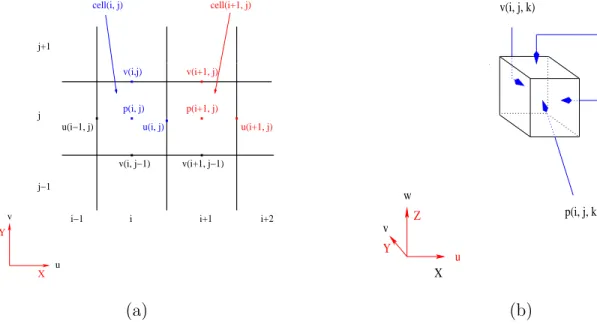
The nx×ny×nz domain in Figure 3.1 is discretized as a staggered grid, in which the different unknown variables are not located at the same grid points [17]. For example, as demonstrated in Figure 3.6, for a particular cell in 3D, pressure p is located in the cell center while u, v and w are at the center of the right, back and top planes of that cell respectively,i.e., the location ofu,v andwall shift by half a cell length along the positive coordinate directions accordingly. This staggered arrangement of the unknowns prevents possible pressure oscillations which could occur if we evaluate all unknown values of u,v,

w andpat the same grid points. But it should be noted that not all extremal grid points lie on the domain boundaries. For instance, in Figure 3.6(a), the vertical boundaries have

(45)

nov-values, just as the horizontal boundaries have nou-values. For this reason, an extra boundary strip of grid cells, as shown in Figure 3.7, is introduced, so that the boundary conditions may be applied by averaging the nearest grid points on either side.

v(i+1, j) p(i+1, j)

u(i+1, j)

u

v i−1 i+1 i+2

j−1 j j+1 v(i,j) p(i, j) X u(i, j) v(i, j−1) v(i+1, j−1) u(i−1, j) Y cell(i, j) cell(i+1, j) i u(i, j, k) w(i, j, k) v(i, j, k) p(i, j, k) w v X Y Z u (a) (b)

Figure 3.6: Staggered grid applied in 2D and 3D. (a) In 2D, velocities (u, v) and pressure (p) are in different locations on the plane. (Redrawn from Griebel et al. [17]). (b) In 3D, velocities (u, v, w) shift by half a cell length along the positive X, Y and Z coordinate directions and they locate at the cell boundary plane centers while pressure (p) is at the cell center.

The numerical treatment on boundary with different boundary condtions is described as follows [17]. To simplify the discussion, the explanation is given in 2D based on the diagrams presented in Figure 3.6(a) and Figure 3.7.

In order to formulate the boundary conditions, we first define the following notations as introduced in [17]:

(46)

3.3. NUMERICAL SOLUTION

boundary strip boundary of domain

v(1,0) j=jmax+1 j=jmax j=2 j=1 j=0

i=0 i=1 i=2 i=imax i=imax+1

v(0,1) v(1,1) u(1,1) u(0,1) u(0,0) v u Y X

Figure 3.7: Staggered arrangement of the unknowns on a 2D domain after an extra boundary strip of grid cells is introduced (Redrawn from [17]).

direction).

ϕt: the component of velocity parallel to the boundary (in the tangential direction).

∂ϕn

∂n : the first derivative ofϕn (in the normal direction). ∂ϕt

∂n: the first derivative of ϕt (in the normal direction).

Then, along the vertical boundary segments, i.e., along the Y direction in Figure 3.6(a) and Figure 3.7, we have

ϕn=u, ϕt=v, ∂ϕn ∂n = ∂u ∂x, ∂ϕt ∂n = ∂v ∂x (3.2)

(47)

and, along the horizontal segments, i.e., along the X direction in Figure 3.6(a) and Figure 3.7, ϕn =v, ϕt=u, ∂ϕn ∂n = ∂v ∂y, ∂ϕt ∂n = ∂u ∂y (3.3)

So for cells on the boundary, different boundary conditions can be implemented as follows [17]:

1. no-slip condition, i.e.,

ϕn(x, y) = 0, ϕt(x, y) = 0

by

u0,j = 0, uimax,j = 0, j = 1, ..., jmax

vi,0 = 0, ui,jmax = 0, i= 1, ..., imax

v0,j =−v1,j, vimax+1,j =−vimax,j, j = 1, ..., jmax

ui,0 =−ui,1, ui,jmax+1 =−ui,jmax, i= 1, ..., imax

In this simulation, this condition is applied to u, v and w on the bottom boundary as shown in Figure 3.1.

2. free-slip condition, i.e.,

ϕn(x, y) = 0,

∂ϕt(x, y)

(48)

3.3. NUMERICAL SOLUTION

by

u0,j = 0, uimax,j = 0, j = 1, ..., jmax

vi,0 = 0, ui,jmax = 0, i= 1, ..., imax

v0,j =v1,j, vimax+1,j =vimax,j, j = 1, ..., jmax

ui,0 =ui,1, ui,jmax+1 =ui,jmax, i= 1, ..., imax

In this simulation, this condition is applied to won the 4 vertical boundary planes, as well as u and v on the top boundary.

3. inflow condition,i.e.,

ϕn(x, y) =ϕn0, ϕt(x, y) = (ϕt)0, ϕn0, (ϕt)0 given

As the definition of inflow condition is that the velocities are explicitly given on the inflow boundary, for the velocities normal to the boundary (e.g., u on the left boundary), we can set the values on the boundary; for the velocity components tangential to the boundary (e.g., v on the left boundary), we assign the values by averaging the values on either side of the boundary. In the simulation here, this condition is applied to u and v on the 4 vertical boundary planes, and the values assigned on the boundary are based on the shear flow profile shown in Figure 3.4(b).

(49)

4. outflow condition, i.e., ∂ϕn(x, y) ∂n = 0, ∂ϕt(x, y) ∂n = 0 by

u0,j =u1,j, uimax,j =uimax−1,j, j = 1, ..., jmax

v0,j =v1,j, vimax+1,j =uimax,j, j = 1, ..., jmax

ui,0 =ui,1, ui,jmax+1 =ui,jmax, i= 1, ..., imax

vi,0 =vi,1, vi,jmax =vi,jmax−1, i= 1, ..., imax

In the simulation, this condition is only applied to w on the top boundary. As the staggered arrangement shown in Figure 3.6(b), w lies on the top boundary. So for a particular boundary cell on the top, its w value is first assigned based on the velocity magitude function (3.1) presented in Section 3.1, then its neighbor inside the domain is set having the same wvalue.

Finally, the equations are solved by using finite difference method. Interested readers can find detailed explanations in Chapter 3 of [17]. The outline of the equation solving algorithm is that Conjugate-gradient method is used to solve the Possion equation for pressurep at timet given the velocitiesu, v and wat time t₋1. Then, the newu,v and

(50)

Chapter 4

Rendering Algorithm

How to visualize the simulated tornado flow is discussed in this chapter. In Section 4.1, the particle system theory and the system used in this simulation are introduced first. The purpose of using a particle system in this thesis is to define the tornado volume which is difficult to be represented by using the classical geometric elements, such as polygons. Then in Section 4.2, the particle density calculation and density smoothing techniques applied in this simulation are discussed, with the volume rendering algorithm being introduced at the end.

(51)

4.1

Particle System

4.1.1

Overview

In computer graphics, the generation of objects or structures procedurally1_{is an important}

area, and functionally based modeling2 methods are generally applied in 3D computer graphics to achieve this goal. Among them, three most important techniques applied are discussed in [42]:

• non-deterministic or stochastic functions. They are used to represent a particular subject with randomness. In computer graphics, terrain, fire and turbulence have been generated by using such random functions.

• deterministic functions. Randomness is not involved, so such functions can produce the same output given the fixed initial conditions.

• the functions which involve both randomness and non-randomness, i.e., the combi-nation of the above two.

In 3D computer graphics, these techniques are widely used for modeling purpose to pro-duce objects. For example, in natural phenomena simulation, they have been used to generate particles to model fuzzy objects, such as clouds and smoke [32]. These objects do not have smooth and “well-defined” shapes and are dynamic, so it is difficult to rep-resent them using the classical “surface-based” elements such as polygons or patches. In

1_{Graphical image is generated from programming code but not picture files [42].}

2_{To generate objects or structures procedurally, the computer program code is composed of several}

functions to produce the rendered image step by step. This is called functionally based modeling in computer graphics [42].

(52)

4.1. PARTICLE SYSTEM

these cases, particle systems are applied to model such fuzzy ojects. A particle system models these objects as “a cloud of primitive particles that define their volume”, and particles can move over time. Therefore, a particle system is able to represent the object movement and shape changes, thus images with irregular or “ill-defined” object shapes can be generated without applying a complicated geometry system.

In a particle system, depending on the object being modeled, a particle may have varied attributes. But in general, a particle has the following characteristics [15, 32, 42]: position, mass, velocity (both speed and direction), size, color, transparency, shape and lifetime. Over the time, new particles are generated into the system and their attributes are initialized, then these attributes are modified at later time steps to represent the shape and dynamic movement of the modeled object. Finally, when particles reach their lifetime they die and are out of the system.

The general framework of a particle system can be decribed as [15, 32]:

1. new particles are generated into the system,

2. each new particle is assigned initial attribute values,

3. all particles that reach their lifetime are out of the system,

4. all remaining particles update their attributes at each time step, and

5. an image of the existing particles is rendered.

As discussed in [32], such system can be implemented using a computer language to execute several functions. In computer graphics, simple stochastic (non-deterministic)

(53)

processes are generally used to generate particles. To control the shape, appearance and dynamics of particles, the model designer needs to assign a set of parameters to control the range of randomness. On the other hand, because such modeling process is procedural, the modeling steps can also incorporate other computational model solutions which describe the dynamics of the object. For example, the solution of a partial differential equations could be tied to a particle system to provide the particle attribute information. This is the approach applied in this tornado simulation which will be discussed next.

Of course, a static object can be also represented using the modeling process of a particle system, but such modeling process is more interesting when it is used to model the “time-varying” phenomena for animation purpose [42]. This technique has been used in computer graphics to simulate natural phenomena. For example, in addition to clouds and smoke introduced earlier, fire and explosions have also been modeled using particle systems, as presented in the filmStar Trek II: The Wrath of Khanin June, 1982 and Return of the Jedi in May, 1983 [32]. Moreover, aurora [1] has been simulated by using a particle-mesh method and grass [32] has been simulated as well by using a partially stochastic technique. One important aspect of particle systems is that particles can move. Thus many other natural phenomena can also be simulated by using particle systems to represent their dynamics, such as the tornado simulation here.

4.1.2

The Particle System in this Simulation

The shape diversity and flow dynamics of tornadoes make their geometry description difficult, thus it is hard to define their volume using the classical geometric elements,

(54)

4.1. PARTICLE SYSTEM

but a particle system makes it possible to model their volume and dynamics over time. Moreover, it is believed that particle density directly relates to transparency, so a coupled particle system is applicable to the realistic visual result. For example, in the filmTWISTER

[10] released in 1996, particle systems are used to simulate the tornado movement and shape changes. In their particle systems, a particle has position, lifetime, velocity, acceler-ation, color and transparency attributes. Randomness based functions are used to update such attributes. So their simulation is for pure visual purpose without taking into account the physical characteristics in the tornado evolution process, but in this simulation, the partical attributes are updated based on the solutions of physical model equations which is physically-based at some extent.

In the particle system of this simulation, a particle has position, lifetime, velocity and mass attributes. The initial position of a particle depends on the purpose of such particle. For example, at the beginning of the simulation, certain number of particles are added into the system at random positions to describe how the cube shape converges to a particular tornado shape at the end. But some other particles are added at later steps at specific locations to simulate some other effects, such as color variation and bottom debris swirling effect. The lifetime attribute is defined by the position instead of time as a particle system usually does. For example, during the simulation, a particle dies if it is out of the system boundaries, otherwise, its position is updated based on its velocity (speed and direction). As presented earlier, this particle system is coupled with the model’s numerical solutions. So at each time step, the position attribute is updated based on the velocity solutions instead of using random process as generally applied in computer graphics. Therefore, to simulate a particular tornado shape, the particle positions can

(55)

be controlled accordingly by applying appropriate boundary conditions. One example is given here to show how this process works in this simulation, such as how the attributes are initialized and how they are updated. In Figure 5.2(a) of Chapter 5, a simulated funnel shape tornado is presented. In order to produce such particular shape, the boundary conditions and velocity magitude control functions decribed in Section 3.2 are applied to compute velocity solutions. Then a particle system is integrated with the equation solver. To simulate the tornado evolving process, 500000 particles are randomly generated at the beginning to fill the whole domain. After that, at each time step, 1200 new particles are generated into the system only at the bottom3 _{in order to fill the} _hole_{, which is caused by}

the upward particles generated at earlier steps. So depending on the purpose, particles have different initial positions. Then all the living particles move based on their current positions and the velocity information computed from the numerical solutions. Thus after rendering, an interesting tornado shape is produced, and finally the wind flow movement, such as rotation and going up, is observed in the animation.

Moreover, to simulate the debris swirling effect at tornado bottom, some special par-ticles are generated at each time step. In the simulation presented in Figure 5.4(b), 40 special particles are generated into the system at each step. All these particles have mass attribute. Note that the particles discussed above do not have mass attributes due to the assumption that only the water vapor, which does not have mass, is in the wind. But this assumption cannot be applied to simulate the debris swirling effect at bottom because clearly debris has mass. In the simulation, the mass value is randomly initialized when the particle enters the system. Then, by applying gravity and centrifugal force, the

3_{On the plane of}

(56)

4.1. PARTICLE SYSTEM

velocity attribute of these particles is modified differently from the numerical solutions. The details are discussed next.

At time stepn, for a particular particle for debris swirling effect simulation, it has the following attribute denotions:

1. position: (xn_{, y}n_),

2. velocity: (un_{, v}n_{), and}

3. mass: m

Moreover, as the simulated rotation is expected to be counter-clockwise, the velocity of this particle is illustrated in component form accordingly in Figure 4.1(a). We also know that, by Newton’s first and third law of motion, the magitude of centrifugal force of this particle can be computed by

F =m v

2

r ,

where v is this particle’s velocity, r is the rotation radius, i.e., the distance from point (xc, yc) to (xn, yn) in Figure 4.1. In this simulation, this formula is rewritten as

Fn=m (u n₎2_{+ (}_vn₎2 p (xn₋_x c)2+ (yn−yc)2 (4.1)

The angle ofβshown in Figure 4.1 can be calculated based on the formula arctan(|_|v_unn|_|).

Thus, the X and Y components of Fn _{can be given as} _Fn

x = Fn · sin(β) and Fyn =

Fn

·cos(β), respectively. Their geometry relationship is shown in Figure 4.1(b). Because the acceleration an ₌ Fn

m, we have the value of its X component a n

x =

Fn

x m

(57)

c, yc) (x (xn_{, y}n₎ X Y v u un vn Velocity c, yc) (x (xn_{, y}n₎ ß ß X Y v u F Fn y n Fn (a) (b) x

Figure 4.1: The decomposition of velocity and centrifugal force for a particular particle in the bottom debris swirling simulation. (a) Velocity decomposition. (b) Centrifugal force decomposition.

(58)