Penetration Rate Optimization With Support Vector Regression Method

(1)

ISTANBUL TECHNICAL UNIVERSITY  GRADUATE SCHOOL OF SCIENCE ENGINEERING AND TECHNOLOGY

M.Sc. THESIS

JUNE 2015

PENETRATION RATE OPTIMIZATION WITH SUPPORT VECTOR REGRESSION METHOD

Korhan KOR

Department of Petroleum and Natural Gas Engineering Petroleum and Natural Gas Engineering Programme

(2)

(3)

JUNE 2015

ISTANBUL TECHNICAL UNIVERSITY  GRADUATE SCHOOL OF SCIENCE ENGINEERING AND TECHNOLOGY

PENETRATION RATE OPTIMIZATION WITH SUPPORT VECTOR REGRESSION METHOD

M.Sc. THESIS

Department of Petroleum and Natural Gas Engineering Petroleum and Natural Gas Engineering Programme

Korhan KOR (505121501)

(4)

(5)

HAZİRAN 2015

DESTEK VEKTÖR REGRESYONU YÖNTEMİ İLE İLERLEME HIZI OPTİMİZASYONU

YÜKSEK LİSANS TEZİ Korhan Kor (505121501)

İSTANBUL TEKNİK ÜNİVERSİTESİ  FEN BİLİMLERİ ENSTİTÜSÜ

Petrol ve Doğal Gaz Mühendisliği Anabilim Dalı Petrol ve Doğal Gaz Mühendisliği Programı

(6)

(7)

Thesis Advisor : Asst. Prof. Dr. Gürşat ALTUN ... Istanbul Technical University

Jury Members : Asst. Prof. Dr. Şenol YAMANLAR ... Istanbul Technical University

Prof. Dr. Hanifi ÇOPUR ... Istanbul Technical University

Korhan Kor, a M.Sc. student of ITU Graduate School of Science Engineering and Technology student ID 505121501, successfully defended the thesis entitled “PENETRAION RATE OPTIMIZATION WITH SUPPORT VECTOR REGRESSION METHOD”, which he prepared after fulfilling the requirements specified in the associated legislations, before the jury whose signatures are below.

(8)

(9)

(10)

(11)

FOREWORD

First of all, I would like to thank to my thesis advisor, Asst. Prof. Dr. Gürşat ALTUN for his endless support during my graduate years as a student, a research assistant and an engineer. I also appreciate him for bringing this unique subject of machine learning to me as my thesis topic.

And the second biggest appreciation is for my mother and father, who have raised me, supported me for education, and made me ready for the tough life starting from my childhood. One of the most important contributors of this thesis is my parents, no doubt. Thank you, for everything.

The university and the department have the most important role on me working as a petroleum and natural gas engineer today. So, I would like to thank individually all the professors in the Department of Petroleum and Natural Gas Engineering in Istanbul Technical University. Also, many thanks to my co-workers in the department during my research assistant years, Ali Ettehadi OSGOUEI, Dr. E. Didem KORKMAZ BAŞEL, Eda AY DİLSİZ, F. Bahar HOŞGÖR, Kağan KUTUN, Dr. M. Hakan ÖZYURTKAN, Melek DENİZ PAKER, and Dr. Yıldıray PALABIYIK.

I also would like to thank to Asst. Prof. Dr. Yusuf YASLAN for letting me listen to his “Machine Learning” lectures and helping me for my questions.

Cengiz BERKÜN, Cenk ŞANLIOĞLU and Mert Can SELÇUK… Thank you for being a big brother for me. Thank you for always being there for me. Do not let your music end. We will always be together.

And finally, Ezgi BİLGİÇ… Thank you for always being on my side, for your huge support, for your big heart, and for your love.

May 2015 Korhan KOR

(12)

(13)

TABLE OF CONTENTS Page FOREWORD ... ix TABLE OF CONTENTS ... xi ABBREVIATIONS ... xiii LIST OF TABLES ... xv

LIST OF FIGURES ... xix

SYMBOLS ... xxiii

SUMMARY ... xxv

ÖZET ... xxvii

1. INTRODUCTION ... 1

2. LITERATURE REVIEW ... 7

2.1 Former Studies on ROP Optimization ... 7

2.2 Recent Studies on ROP Optimization ... 17

3. STATEMENT OF THE PROBLEM AND SCOPE OF THE THESIS ... 31

4. MULTIPLE REGRESSION AND BOURGOYNE & YOUNG METHOD ... 35

4.1 Theory of Multiple Regression Analysis ... 35

4.1.1 Introduction to multiple regression analysis ... 35

4.1.2 Least squares estimation of the parameters ... 36

4.1.3 Matrix approach ... 38

4.2 Bourgoyne and Young Method ... 39

4.2.1 Effect of formation strength ... 40

4.2.2 Effect of normal compaction ... 41

4.2.3 Effect of under compaction ... 41

4.2.4 Effect of overbalance ... 42

4.2.5 Effect of bit weight and bit diameter ... 43

4.2.6 Effect of rotary speed ... 44

4.2.7 Effect of tooth wear ... 45

4.2.8 Effect of bit hydraulics ... 47

5. MACHINE LEARNING AND SUPPORT VECTOR REGRESSION ... 51

5.1 Statistical Learning Theory ... 58

5.1.1 VC dimension ... 59

5.1.2 Structural risk minimisation ... 60

5.2 Support Vector Machines for Classification ... 60

5.2.1 The optimal separating hyperplane ... 62

5.2.2 The generalized optimal separating hyperplane ... 67

5.3 Kernel Functions ... 69

5.3.1 Linear kernels ... 70

5.3.2 Gaussian radial basis function kernels ... 71

5.4 Support Vector Regression ... 71

5.4.1 ε-insensitive regression ... 72

(14)

5.5 Cross Validation and Overfitting ... 76

5.5.1 K-fold cross validation ... 78

5.5.2 Leave-one-out cross validation ... 78

5.6 Toolboxes ... 78

5.6.1 R programming language ... 78

5.6.2 LIBSVM ... 79

5.6.3 e1071 package ... 79

5.7 Statistical Comparison Criteria ... 79

5.7.1 Residual sum of squares ... 80

5.7.2 R2 ... 80

5.7.3 Pseudo-R2_{... 81}

5.7.4 Root mean squared error ... 81

6. RESULTS AND DISCUSSIONS ... 83

6.1 Case 1: Training Top 16 Depth Interval ... 84

6.1.1 Testing #17-18-19-20 ... 84

6.1.2 Testing #22-23-24-25 ... 87

6.1.3 Testing #27-28-29-30 ... 90

6.1.4 Testing #17-21-26-30 ... 93

6.2 Case 2: Training Bottom 16 Depth Interval ... 98

6.2.1 Testing #11-12-13-14 ... 98

6.2.2 Testing #6-7-8-9 ... 101

6.2.3 Testing #1-2-3-4 ... 104

6.2.4 Testing #1-5-10-14 ... 107

6.3 Case 3: Training Odd Numbered Data Points ... 113

6.3.1 Testing #2-4-6-8 ... 113

6.3.2 Testing #12-14-16-18 ... 116

6.3.3 Testing #22-24-26-28 ... 119

6.3.4 Testing #2-10-20-30 ... 122

6.4 Case 4: Training Even Numbered Data Points ... 127

6.4.1 Testing #1-3-5-7 ... 127

6.4.2 Testing #11-13-15-17 ... 130

6.4.3 Testing #21-23-25-27 ... 133

6.4.4 Testing #1-9-19-29 ... 136

6.5 Case 5: Training Several 24 Data Points ... 142

6.5.1 Training first 24, testing last 6 data inputs ... 142

6.5.2 Training last 24, testing first 6 data inputs ... 145

6.5.3 Training mid 24, testing #1-2-3-28-29-30... 148

6.5.4 Training several 24, testing #4-7-10-18-22-27 ... 151

6.6 Case 6: Training All Data Points ... 156

6.6.1 Testing #1-2-3-4-5... 157

6.6.2 Testing #26-27-28-29-30... 160

6.6.3 Testing #14-15-16-17-18... 163

6.6.4 Testing #1-6-11-16-21... 166

6.6.5 Testing all ... 171

6.7 Case 7: Training Different Data Set ... 175

6.8 Discussions and General Interpretations ... 179

7. CONCLUSIONS AND RECOMMENDATIONS ... 181

REFERENCES ... 183

(15)

ABBREVIATIONS

ANN : Artificial Neural Networks BYM : Bourgoyne and Young Model

DENFIS : Dynamic Evolving Neural-Fuzzy Inference System GA : Genetic Algorithm

GDL : Geological Drilling Log KKT : Karush-Kuhn-Tucker LWD : Logging While Drilling ML : Machine Learning

MSE : Mechanical Specific Energy MR : Multiple Regression

MWD : Measurement While Drilling

OCSH : Optimal Canonical Separating Hyperplane PDC : Polycrystalline Diamond Compact

PVT : Pressure Volume Temperature RBF : Radial Basis Function

RKHS : Reproducing Kernel Hilbert Spaces RMSE : Root Mean Squared Error

ROP : Rate of Penetration RSS : Residual Sum of Squares SRM : Structural Risk Minimization SV : Support Vectors

SVM : Support Vector Machines SVR : Support Vector Regression TCC : Tungsten Carbide Core TSS : Total Sum of Squares TVD : Total Vertical Depth VC : Vapnik-Chervonenkis WOB : Weight on Bit

(16)

(17)

LIST OF TABLES

Page

Table 1.1 : Methods of operations research ... 2

Table 4.1 : Data tabulation for multiple regression ... 36

Table 5.1 : Summary of ML settings ... 55

Table 6.1 : Multiple regression coefficients of Case 1 ... 84

Table 6.2 : Statistics of the data set in Case 1 for testing #17-18-19-20 ... 85

Table 6.3 : Statistical results of MR in Case 1 for learning and testing #17-18-19- 20 ... 85

Table 6.4 : Statistical results of the methods in Case 1 for testing #17-18-19-20. ... 85

Table 6.5 : ROP predictions in Case 1 for #17-18-19-20... 85

Table 6.8 : Statistical results of the methods in Case 1 for testing #22-23-24-25 .... 88

Table 6.9 : ROP predictions in Case 1 for #22-23-24-25... 88

Table 6.12 : Statistical results of the methods in Case 1 for testing #27-28-29-30 .. 91

Table 6.13 : ROP predictions in Case 1 for #27-28-29-30 ... 91

Table 6.15 : Statistical results of MR in Case 1 for learning and testing #17-21- 26-30 ... 94

Table 6.16 : Statistical results of the methods in Case 1 for testing #17-21-26-30 .. 94

Table 6.18 : Multiple regression coefficients of Case 2 ... 98

Table 6.21 : Statistical results of the methods in Case 2 for testing #11-12-13-14 100 Table 6.22 : ROP predictions in Case 2 for #11-12-13-14 ... 100

Table 6.24 : Statistical results of MR in Case 2 for learning and testing #6-7-8-9 . 102 Table 6.25 : Statistical results of the methods in Case 2 for testing #6-7-8-9 ... 103

Table 6.28 : Statistical results of MR in Case 2 for learning and testing #1-2-3-4 . 105 Table 6.29 : Statistical results of the methods in Case 2 for testing #1-2-3-4 ... 106

(18)

Table 6.32 : Statistical results of MR in Case 2 for learning and testing #1-5-10-

14 ... 108

Table 6.33 : Statistical results of the methods in Case 2 for testing #1-5-10-14 ... 109

Table 6.40 : Statistics of the data set in Case 3 for testing #12-14-16-18 ... 117

Table 6.41 : Statistical results of MR in Case 3 for testing #12-14-16-18 ... 117

Table 6.42 : Statistical results of the methods in Case 3 for testing #12-14-16-18. 117 Table 6.43 : ROP predictions in Case 3 for #12-14-16-18 ... 117

Table 6.46 : Statistical results of the methods in Case 3 for testing #22-24-26-28. 120 Table 6.47 : ROP predictions in Case 3 for #22-24-26-28 ... 120

Table 6.50 : Statistical results of the methods in Case 3 for testing #2-10-20-30 ... 123

Table 6.52 : Multiple regression coefficients of Case 4. ... 127

Table 6.53 : Statistics of the data set in Case 4 for testing #1-3-5-7 ... 128

Table 6.58 : Statistical results of MR in Case 4 for testing #11-13-15-17 ... 131

Table 6.61 : Statistics of the data set in Case 4 for testing #21-23-25-27 ... 134

Table 6.67 : Statistical results of the methods in Case 4 for testing #1-9-19-29 ... 138

Table 6.69 : Multiple regression coefficients in Case 5 for testing last 6 ... 141

Table 6.70 : Statistics of the data set in Case 5 for testing last 6 ... 143

Table 6.71 : Statistical results of MR in Case 5 for learning and testing last 6 ... 143

Table 6.72 : Statistical results of the methods in Case 5 for testing last 6 ... 143

Table 6.73 : ROP predictions in Case 5 for last 6 ... 143

Table 6.74 : Multiple regression coefficients in Case 5 for testing first 6 ... 145

(19)

Table 6.77 : Statistical results of the methods in Case 5 for testing first 6 ... 146

Table 6.78 : ROP predictions in Case 5 for first 6 ... 146

Table 6.79 : Multiple regression coefficients in Case 5 for testing #1-2-3-28-29- 30 ... 148

Table 6.80 : Statistics of the data set in Case 5 for testing #1-2-3-28-29-30 ... 149

Table 6.81 : Statistical results of MR in Case 5 for learning and testing #1-2-3- 28-29-30 ... 149

Table 6.82 : Statistical results of the methods in Case 5 for testing #1-2-3-28- 29-30 ... 149

Table 6.83 : ROP predictions in Case 5 for #1-2-3-28-29-30 ... 149

Table 6.84 : Multiple regression coefficients in Case 5 for testing #4-7-10-18- 22-27 ... 151

Table 6.85 : Statistics of the data set in Case 5 for testing #4-7-10-18-22-27 ... 152

Table 6.86 : Statistical results of MR in Case 5 for learning and testing #4-7-10- 18-22-27 ... 152

Table 6.87 : Statistical results of the methods in Case 5 for testing #4-7-10-18- 22-27 ... 152

Table 6.88 : ROP predictions in Case 5 for #4-7-10-18-22-27 ... 152

Table 6.90 : Statistics of the data set in Case 6 for testing #1-2-3-4-5 ... 157

Table 6.91 : Statistical results of MR in Case 6 for learning and testing #1-2-3- 4-5 ... 158

Table 6.92 : Statistical results of the methods in Case 6 for testing #1-2-3-4-5 ... 158

Table 6.93 : ROP predictions in Case 6 for #1-2-3-4-5 ... 158

Table 6.94 : Statistics of the data set in Case 6 for testing #26-27-28-29-30 ... 161

Table 6.95 : Statistical results of MR in Case 6 for learning and testing #26-27- 28-29-30 ... 161

Table 6.96 : Statistical results of the methods in Case 6 for testing #26-27-28-29- 30 ... 161

Table 6.99 : Statistical results of MR in Case 6 for learning and testing #14-15- 16-17-18 ... 164

Table 6.100 : Statistical results of the methods in Case 6 for testing #14-15-16- 17-18 ... 164

Table 6.101 : ROP predictions in Case 6 for #14-15-16-17-18 ... 164

Table 6.103 : Statistical results of MR in Case 6 for learning and testing #1-6-11- 16-21 ... 167

Table 6.104 : Statistical results of the methods in Case 6 for testing #1-6-11-16- 21 ... 167

Table 6.106 : Statistics of the data set in Case 6 for testing all ... 171

Table 6.107 : Statistical results of MR in Case 6 for learning and testing all ... 171

Table 6.108 : Statistical results of the methods in Case 6 for testing all ... 172

Table 6.109 : ROP predictions in Case 6 for all ... 173

Table 6.110 : Statistics of the data set in Case 7 for testing all ... 175

Table 6.111 : Multiple regression coefficients in Case 7 for testing all ... 176

Table 6.112 : Statistical results of MR in Case 7 for learning and testing all ... 176

(20)

Table 6.114 : ROP predictions in Case 7 for all ... 177 Table A.1: The main data set ... 199 Table A.2: The recent data set ... 201

(21)

LIST OF FIGURES

Page

Figure 1.1 : Minimum and maximum of a function ... 1

Figure 1.2 : An example of time and cost relationship ... 4

Figure 2.1 : Optimum WOB and rotary speed ... 15

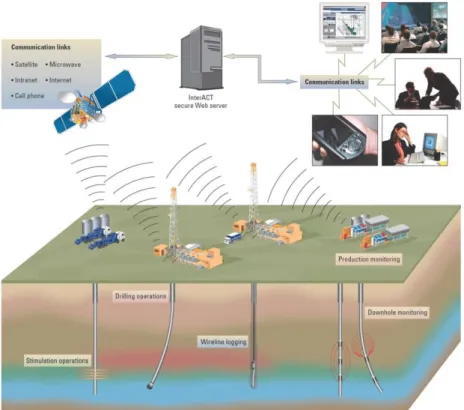
Figure 2.2 : The InterACT system ... 18

Figure 2.3 : Algorithm of the mathematical optimization procedure ... 24

Figure 2.4 : Hole cleaning chart example ... 25

Figure 2.5 : Flowchart of a soft computing approach ... 26

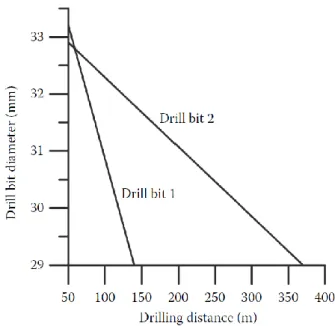
Figure 2.6 : Decrease in drill bit diameter via wear characteristics ... 29

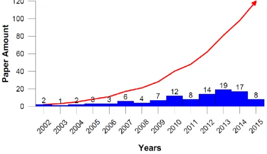
Figure 2.7 : Number of papers including SVM found in OnePetro database. ... 30

Figure 4.1 : Functional relationship of penetration rate. ... 40

Figure 4.2 : Effect of normal compaction on ROP ... 41

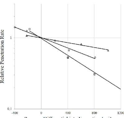
Figure 4.3 : Effect of differential bottom-hole pressure on ROP... 42

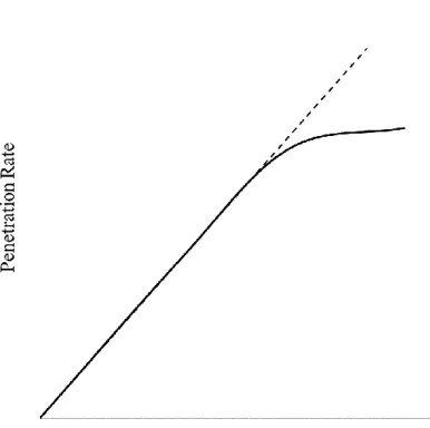
Figure 4.4 : Typical response of penetration rate to increasing bit weight ... 43

Figure 4.5 : Typical response of penetration rate to increasing rotary speed ... 45

Figure 4.6 : Effect of tooth wear on penetration rate ... 46

Figure 4.7 : Tooth wear chart for a roller-cone bit... 47

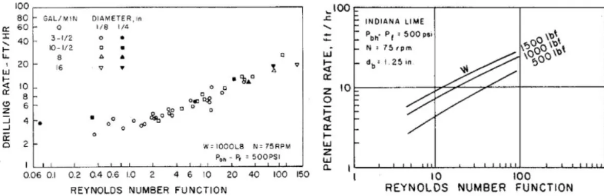
Figure 4.8 : ROP as a function of bit Reynolds number ... 47

Figure 4.9 : The effect of different hydraulic models on ROP ... 48

Figure 5.1 : Expert Systems flowchart ... 52

Figure 5.2 : Genetic Algorithms flowchart ... 53

Figure 5.3 : Fuzzy Logic flowchart ... 53

Figure 5.4 : Machine Learning related fields ... 54

Figure 5.5 : An overview of how ML works ... 54

Figure 5.6 : An example of linear classification in two dimensions ... 55

Figure 5.7 : An example of decision tree ... 56

Figure 5.8 : Mapping of ML methods ... 57

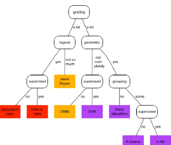
Figure 5.9 : ML taxonomy ... 58

Figure 5.10 : Modelling errors ... 59

Figure 5.11 : VC dimension illustration... 59

Figure 5.12 : Classifier examples ... 61

Figure 5.13 : Linear classification... 61

Figure 5.14 : Optimal canonical seperating hyperplane ... 63

Figure 5.15 : Canonical hyperplanes and constraints ... 64

Figure 5.16 : Generalized optimal separating hyperplane ... 67

Figure 5.17 : Feature space illustration ... 69

Figure 5.18 : Loss functions ... 71

Figure 5.19 : ε-insensitive loss function and slack variables ... 73

Figure 5.20 : Overfitting example ... 76

Figure 5.21 : Reducing overfitting ... 77

(22)

Figure 6.2 : ROP prediction trends in Case 1 for testing #17-18-19-20 ... 86 Figure 6.3 : ROP prediction comparison in Case 1 for testing #27-28-29-30 ... 86 Figure 6.4 : Cost graphics of Case 1 for testing #22-23-24-25 ... 87 Figure 6.5 : ROP prediction trends in Case 1 for testing #22-23-24-25 ... 89 Figure 6.6 : ROP prediction comparison in Case 1 for testing #22-23-24-25 ... 89 Figure 6.7 : Cost graphics of Case 1 for testing #27-28-29-30 ... 90 Figure 6.8 : ROP prediction trends in Case 1 for testing #27-28-29-30 ... 92 Figure 6.9 : ROP prediction comparison in Case 1 for testing #27-28-29-30 ... 92 Figure 6.10 : Cost graphics of Case 1 for testing #17-21-26-30 ... 93 Figure 6.11 : ROP prediction trends in Case 1 for testing #17-21-26-30 ... 95 Figure 6.12 : ROP prediction comparison in Case 1 for testing #17-21-26-30 ... 95 Figure 6.13 : RSSmodel values for Case 1 ... 96

Figure 6.14 : CV error values for Case 1 ... 97 Figure 6.15 : Testing errors for Case 1 ... 97 Figure 6.16 : Pseudo-R2 values for Case 1 ... 98 Figure 6.17 : Cost graphics of Case 2 for testing #11-12-13-14 ... 99 Figure 6.18 : ROP prediction trends in Case 2 for testing #11-12-13-14 ... 99 Figure 6.19 : ROP prediction comparison in Case 2 for testing #11-12-13-14 ... 101 Figure 6.20 : Cost graphics of Case 2 for testing #6-7-8-9 ... 102 Figure 6.21 : ROP prediction trends in Case 2 for testing #6-7-8-9 ... 103 Figure 6.22 : ROP prediction comparison in Case 2 for testing #6-7-8-9 ... 104 Figure 6.23 : Cost graphics of Case 2 for testing #1-2-3-4 ... 105 Figure 6.24 : ROP prediction trends in Case 2 for testing #1-2-3-4 ... 106 Figure 6.25 : ROP prediction comparison in Case 2 for testing #1-2-3-4 ... 107 Figure 6.26 : Cost graphics of Case 2 for testing #1-5-10-14 ... 108 Figure 6.27 : ROP prediction trends in Case 2 for testing #1-5-10-14 ... 109 Figure 6.28 : ROP prediction comparison in Case 2 for testing #1-5-10-14 ... 110 Figure 6.29 : RSSmodel values for Case 2 ... 111

Figure 6.30 : CV error values for Case 2 ... 111 Figure 6.31 : Testing errors for Case 2 ... 112 Figure 6.32 : Pseudo-R2_{values for Case 2 ... 112}

Figure 6.33 : Cost graphics of Case 3 for testing #2-4-6-8 ... 113 Figure 6.34 : ROP prediction trends in Case 3 for testing #2-4-6-8 ... 115 Figure 6.35 : ROP prediction comparison in Case 3 for testing #2-4-6-8 ... 115 Figure 6.36 : Cost graphics of Case 3 for testing #12-14-16-18 ... 116 Figure 6.37 : ROP prediction trends in Case 3 for testing #12-14-16-18 ... 118 Figure 6.38 : ROP prediction comparison in Case 3 for testing #12-14-16-18 ... 118 Figure 6.39 : Cost graphics of Case 3 for testing #22-24-26-28 ... 119 Figure 6.40 : ROP prediction trends in Case 3 for testing #22-24-26-28 ... 121 Figure 6.41 : ROP prediction comparison in Case 3 for testing #22-24-26-28 ... 121 Figure 6.42 : Cost graphics of Case 3 for testing #2-10-20-30 ... 122 Figure 6.43 : ROP prediction trends in Case 3 for testing #2-10-20-30 ... 124 Figure 6.44 : ROP prediction comparison in Case 3 for testing #2-10-20-30 ... 124 Figure 6.45 : RSSmodel values for Case 3 ... 125

Figure 6.46 : CV error values for Case 3 ... 126 Figure 6.47 : Testing errors for Case 3 ... 126 Figure 6.48 : Pseudo-R2_{values for Case 3 ... 127}

Figure 6.49 : Cost graphics of Case 4 for testing #1-3-5-7 ... 128 Figure 6.50 : ROP prediction trends in Case 4 for testing #1-3-5-7 ... 129

(23)

Figure 6.52 : Cost graphics of Case 4 for testing #11-13-15-17 ... 131 Figure 6.53 : ROP prediction trends in Case 4 for testing #11-13-15-17 ... 132 Figure 6.54 : ROP prediction comparison in Case 4 for testing #11-13-15-17 ... 133 Figure 6.55 : Cost graphics of Case 4 for testing #21-23-25-27 ... 134 Figure 6.56 : ROP prediction trends in Case 4 for testing #21-23-25-27 ... 135 Figure 6.57 : ROP prediction comparison in Case 4 for testing #21-23-25-27 ... 136 Figure 6.58 : Cost graphics of Case 4 for testing #1-9-19-29 ... 137 Figure 6.59 : ROP prediction trends in Case 4 for testing #1-9-19-29 ... 138 Figure 6.60 : ROP prediction comparison in Case 4 for testing #1-9-19-29 ... 139 Figure 6.61 : RSSmodel values for Case 4 ... 140

Figure 6.62 : CV error values for Case 4 ... 140 Figure 6.63 : Testing errors for Case 4 ... 141 Figure 6.64 : Pseudo-R2 values for Case 4 ... 141 Figure 6.65 : Cost graphics of Case 5 for testing last 6 ... 142 Figure 6.66 : ROP prediction trends in Case 5 for testing last 6 ... 144 Figure 6.67 : ROP prediction comparison in Case 5 for testing last 6 ... 144 Figure 6.68 : Cost graphics of Case 5 for testing first 6 ... 145 Figure 6.69 : ROP prediction trends in Case 5 for testing first 6 ... 147 Figure 6.70 : ROP prediction comparison in Case 5 for testing first 6 ... 147 Figure 6.71 : Cost graphics of Case 5 for testing #1-2-3-28-29-30 ... 148 Figure 6.72 : ROP prediction trends in Case 5 for testing #1-2-3-28-29-30 ... 150 Figure 6.73 : ROP prediction comparison in Case 5 for testing #1-2-3-28-29-30 . 150 Figure 6.74 : Cost graphics of Case 5 for testing #4-7-10-18-22-27 ... 151 Figure 6.75 : ROP prediction trends in Case 5 for testing #4-7-10-18-22-27 ... 153 Figure 6.76 : ROP prediction comparison in Case 5 for testing #4-7-10-18-22-27 153 Figure 6.77 : RSSmodel values for Case 5 ... 154

Figure 6.78 : CV error values for Case 5 ... 155 Figure 6.79 : Testing errors for Case 5 ... 155 Figure 6.80 : Pseudo-R2 values for Case 5 ... 156 Figure 6.81 : Cost graphics of Case 6 for testing #1-2-3-4-5 ... 157 Figure 6.82 : ROP prediction trends in Case 6 for testing #1-2-3-4-5 ... 159 Figure 6.83 : ROP prediction comparison in Case 6 for testing #1-2-3-4-5 ... 159 Figure 6.84 : Cost graphics of Case 6 for testing #26-27-28-29-30 ... 160 Figure 6.85 : ROP prediction trends in Case 6 for testing #26-27-28-29-30 ... 162 Figure 6.86 : ROP prediction comparison in Case 6 for testing #26-27-28-29-30 . 162 Figure 6.87 : Cost graphics of Case 6 for testing #14-15-16-17-18 ... 163 Figure 6.88 : ROP prediction trends in Case 6 for testing #14-15-16-17-18 ... 165 Figure 6.89 : ROP prediction comparison in Case 6 for testing #14-15-16-17-18 . 165 Figure 6.90 : Cost graphics of Case 6 for testing #1-6-11-16-21 ... 166 Figure 6.91 : ROP prediction trends in Case 6 for testing #1-6-11-16-21 ... 168 Figure 6.92 : ROP prediction comparison in Case 6 for testing #1-6-11-16-21 ... 168 Figure 6.93 : RSSmodel values for Case 6 ... 169

Figure 6.94 : CV error values for Case 6 ... 170 Figure 6.95 : Testing errors for Case 6 ... 170 Figure 6.96 : Pseudo-R2 values for Case 6 ... 171 Figure 6.97 : Cost graphics of Case 6 for testing all ... 172 Figure 6.98 : ROP prediction trends in Case 6 for testing all ... 174 Figure 6.99 : ROP prediction comparison in Case 6 for testing all ... 175 Figure 6.100 : Cost graphics of Case 7 for testing all ... 176 Figure 6.101 : ROP prediction trends in Case 7 for testing all ... 178

(24)

(25)

SYMBOLS

AB : Borehole area

Abed : Area of cuttings bed

Awell : Area of the well

Aυ : Projected area of each diamond

Aυw : Projected area of worn section of a diamond

C : Complexity parameter

Cc : Cuttings concentration for a stationary bed

Cf : Formation drillability parameter

D : Well depth E : Rock hardness Es : Specific energy

Fj : Jet impact force

Fjm : Modified jet impact force

H : Normalized bit tooth height K : Drillability of formation K(x,x´) : Kernel function

L(y,f(x)): Loss function M : Margin N : Rotary speed

Ns : Number of diamond stress

Q : Volumetric flow rate R : Rate of penetration Remp[f] : Empirical risk function

Rn : Normalized rate of penetration

R2 _{: Confidence level}

S : Confined rock strength Sc : Compressive strength

T : Bit torque

V : Volume of the rock removal W : Weight on bit Wb : Bit weight Wf : Wear function b : Bias db : Bit diameter dbe : Bearing diameter

dn : Bit nozzle diameter

e : Residual

em : Mechanical efficiency

fc(Pe) : Chip holddown function

gp : Pore pressure gradient

(26)

l : Number of training data

m : Number of insert penetrations per revolution

ni : Number of insert in contact with the rock at the bottom

p : Differential pressure

pc : Circulating bottomhole pressure

pp : Pore pressure

vactual : Mud velocity in annulus

vcritical : Mud critical velocity in annulus

t : Time

w : Weight vector ŷ : Predicted value y̅ : Mean value Φ : Lagrangian

α,β,η : Lagrange multipliers γ : RBF kernel parameter γf : Fluid specific gravity

ε : SVR tolerance control parameter

ζ : Bit-specific coefficient of sliding friction λ : Rotary speed exponent

μ : Plastic viscosity ρ : Mud density

ρc : Equivalent circulating density

σp : Ultimate strength of rock at a differential pressure υ : SVR controller parameter

υk : Kinematic viscosity

ξ : Slack variables ψ : Chip formation angle

(27)

PENETRATION RATE OPTIMIZATION WITH SUPPORT VECTOR REGRESSION METHOD

SUMMARY

Drilling operations constitute the major part of the exploration costs. During operations, drill bits are the primary part needs to be changed frequently due to its quick wearing nature. In order to reduce the drilling cost, the optimum bit pulling time must be determined. To determine the optimum bit pulling time, either rate of penetration or the tooth wearing parameter must be estimated. The most common method that developed for estimating the optimum time for bit change is “Bourgoyne and Young” method. In this method, eight parameter coefficients are needed. To obtain these coefficients, thirty different data which can be taken from either different shale zones inside thirty different wells in a field or thirty different shale points from one well is needed. However, when there is not enough data taken from thirty different shale sections, the accuracy of “Bourgoyne and Young” method decreases.

To construct the functional relationship with the data and parameter coefficients, a regression analysis must be performed. In this study, two kind of regression technique is used and the results are compared to each other. First technique is the multiple regression analysis, which is also used in “Bourgoyne and Young” method. This analysis applies least-squares-principled-regression to the data and calculates the parameter coefficients in order to estimate the target function. The second technique is one of different types of machine learning algorithms, called Support Vector Regression. In this technique, first, the data is divided into train and test datasets. Then, the regression model is constructed by using train datasets. At last, the model is applied to test datasets in order to predict the target values for the function.

For the calculations, the selection of training and testing data sets are divided into cases with different scenarios. The results of different predictor methods for each scenario are compared with each other in the corresponding case. The results show the significant effect of data selection on the accuracy of penetration rate prediction. One of the most powerful methods in machine learning, Support Vector Regression, is used for rate of penetration optimization for the first time in the literature with this thesis study. In this way, the chance for further investigations and studies on the practicability of Support Vector Regression on penetration rate optimization is created.

(28)

(29)

DESTEK VEKTÖR REGRESYONU YÖNTEMİ İLE İLERLEME HIZI OPTİMİZASYONU

ÖZET

Günümüzde enerji kaynaklarına olan talep artışı nedeniyle petrol, gaz ve jeotermal kaynak arayışları önemini daha da arttırarak korumaktadır. Bu talep artışını karşılamak amacıyla daha önce araştırma yapılmamış yeraltı derinliklerinde ve su derinliğinin 3000 metreyi bulduğu açık denizlerde yeni kaynak araştırmaları devam etmektedir. Bu araştırma giderlerinin büyük bir çoğunluğunu sondaj operasyonları oluşturmaktadır. Doğası gereği, sondaj esnasında kulenin ve sondaj dizisinin en çok aşınmaya uğrayan, çabuk eskiyip değiştirilmesine ihtiyaç duyulan elemanı matkaptır. Sondajın metraj veya perfornas maliyetini düşürmek için bir matkabın hem uzun süre çalışması, hem de iyi iş yapması istenir. Matkap çalıştıkça aşınacağı için ilerleme hızı azalır ve sondaj maliyeti artmaya başlar. Bu sebepten dolayı, matkabın aşınma durumunun dikkatle takip edilmesi gerekmektedir. Eğer matkap zamanından önce kuyudan çıkarılırsa, başka kuyularda tekrar kullanılma özelliğini çoğunlukla kaybeder. Eğer matkap fazla aşınır ve bu durum fark edilmezse, bazı kısımları (diş, kon, vs.) parçalanarak kuyunun içinde kalır. Bu kalan parçalar çıkarılıp kuyu temizlenmeden sondaja devam edilemeyeceği için tahlisiye olarak adlandırılan kurtarma operasyonlarının yapılmasını zorunlu kılar. Bu durum, zaman ve para kaybına yol açtığı gibi tahlisiye operasyonunun yüzde yüz başarı ile gerçekleşeceğinin garantisi de yoktur.

Sondaj esnasındaki ilerleme hızı birçok parametreye bağlıdır. Bu sebeple, ilerleme hızını tahmin veya optimize etmek oldukça karışıktır. Ancak yaygın optimizasyon yöntemleri kullanılarak, oyma dişli matkaplar için en iyi parametre kombinasyonlarının seçilmesiyle en düşük maliyeti oluşturan matematiksel modeller türetilmiştir. Bu matematiksel modellerden en kapsamlı ve en yaygın olanı Bourgoyne ve Young (BY) yöntemidir. BY yönteminde en iyi ilerleme hızını tahmin edebilmek için sekiz parametre içeren en az otuz girdi veri setine ihtiyaç vardır. Bu otuz veri seti, ya bir sahadaki otuz farklı kuyudan ayrı ayrı şeyl zonlarından alınmış olmalı ya da bir kuyuda otuz farklı derinlikteki şeyl noktalarından elde edilmiş olmalıdır. Herhangi bir sebeple elde yeterli veri olmadığı durumlarda BvY yönteminin doğruluğu azalmakta ve önemli hatalara yol açmaktadır. Bu nedenle, verinin yetersiz olduğu durumlarda alternatif yöntemler kullanılması zorunludur. Bu alternatif yöntemlerden en yaygın olanı, yapay öğrenme yöntemlerinin en etkililerinden biri olan Destek Vektör Regresyonu (DVR)’dur. DVR’nin ilerleme hızı tahmini problemine uygulanabilirliği literatürde ilk kez bu çalışma ile gösterilecektir. Bu çalışmada, ilerleme hızını tahmin etmek için iki farklı regresyon tekniği kullanılmıştır. İlk teknik, BvY’nin uyguladığı çoklu regresyon analizidir. İlerleme hızı probleminde bir bağımlı parametreyi tek bir bağımsız parametre ile bağdaştırmak mümkün değildir. Ayrıca, bu parametreler aynı zamanda birbirlerini de etkilemektedir. Bu nedenle, bu şekilde birden çok parametrenin bulunduğu

(30)

durumlarda tekli regresyon analizi yapmak mümkün olmamaktadır. Çoklu regresyon analizi, parametrelerin birbirleri ile olan ilişkilerini çeşitli yöntemlerle belirleyip, her bir parametre için korelasyon katsayısı hesaplar. Daha sonra bu korelasyon katsayıları sayesinde tahmin modeli oluşturulur. Tahmin modeli oluşturulduktan sonra uygunluk katsayısı adı verilen R2 değeri hesaplanır. Bu sayede katsayıların geçerliliği ve modelin uygunluğu gözlemlenir. R2_{değeri 1’e ne kadar yakınsa}

oluşturulan model o kadar geçerlidir. Çalışmada irdelenmiş olan ilerleme hızı probleminde birbiriyle ilişkili sekiz parametre bulunmaktadır. Her bir sekiz parametre için ise otuz adet veri seti vardır. Bu otuz veri seti, en küçük kareler yöntemi kullanılarak modellenir ve sekiz adet korelasyon katsayısı bulunur.

İkinci teknik ise güçlü bir yapay öğrenme yöntemi olan Destek Vektör Makinesi (DVM)’nin regresyon modelidir. Büyük miktarlardaki verilerin elle işlenmesi ve analizinin yapılması mümkün değildir. Bu tür problemlere çözüm olması amacıyla yapay öğrenme (makine öğrenmesi) yöntemleri geliştirilmiştir. Bu yöntemler, eldeki (geçmiş) verileri kullanarak, bu verilere en uygun modeli bulmaya çalışırlar. Bu işleme, öğrenme işlemi adı verilir. Model oluşturulduktan sonra yeni gelen (gelecek) veriler, bu modele göre analiz edilip sonuç üretilir.

Yapay öğrenme yöntemleri farklı uygulamalara, analizlere ve beklentilere göre gruplara ayrılır. Bu gruplardan en yaygın olanları sınıflandırma, kümeleme ve regresyondur. DVM, sınıflandırma konusunda kullanılan oldukça etkili ve basit yöntemlerden birisidir. DVM’de sınıflandırma işlemi için aynı düzlemde bulunan iki grup, aralarına bir sınır çekilerek birbirinden ayrılır. Sınırın çekileceği yer ise iki grubun da elemanlarına en uzak olan yer olması gerekmektedir. Bu işlem, iki gruba da yakın ve birbirine paralel iki sınır çizgisi çekilerek yapılır. Daha sonra bu sınır çizgileri birbirlerine yaklaştırılarak ortak sınır çizgisi üretilir. DVM’de sınıflandırma işlemi iki grup arasında yapılabileceği gibi ikiden çok grup arasında da yapılabilir. DVM’de regresyon ile sınıflandırma arasında matematiksel olarak çok fark bulunmamaktadır. İki yöntem de yapısal risk minimizasyonu ve istatistiksel öğrenme teorisi ile çalışır. Çıktı olarak sınıflandırma bir çeşit etiket (label) verirken, regresyon bir sayı verir. Bu çalışmada, tahmin edilmesi istenen değer ilerleme hızı, yani sayısal bir değer olduğu için DVM’nin regresyon modeli kullanılmıştır. Bu model Destek Vektör Regresyonu (DVR) olarak adlandırılır. Yöntem, kullanılmak istenen veri setinin öğrenme (train) ve test olmak üzere iki alt veri setlerine bölünmesi ile uygulanır. Öğrenme veri seti kullanılarak, ilgili parametreler ve gözlemler arasındaki ilişki belirlenerek bir regresyon modeli oluşturulur. Daha sonra test veri seti, oluşturulan bu model üzerine uygulanarak hedef değer tahmin edilir.

Bu çalışmada DVR’nin yaygın modellerinden biri olan Epsilon-duyarsız kayıp fonksiyonu ve nü kontrol parametreli model kullanılmıştır. Bu modelde, öğrenme veri setindeki her bir gözlem değerinden en fazla Epsilon kadar sapma yapacak ve mümkün olduğunca düz olacak şekilde bir fonksiyon bulunur. Diğer bir deyişle, Epsilon’dan küçük olan hatalar göz ardı edilir; fakat Epsilon’dan büyük sapmalar kabul edilmez. Belirlenen epsilon bandı civarında da gevşek değerlerin tolare edilebilirliğini belirleyen bir penaltı parametresi belirlenir. υ parametresi ise epsilon bandını kontrol edebilen kullanıcı tarafından belirlenen bir parametredir.

Bu tez çalışmasında DVR yöntemi kullanılarak ilerleme hızı tahminleri BvY çalışmasındaki veri seti kullanımıyla gerçekleştirilmiştir. Veriler sekiz parametre kapsamında tanımlandığı için genel bir yaklaşım olarak parametre sayısının iki katı

(31)

kalan veriler ise test seti olarak kullanılmıştır. Veri seçimi rastgele olabildiği için çok sayıda analiz kombinasyonu ortaya çıkmaktadır. Veri seçiminde tercih edilen yaklaşıma bağlı olarak DVR yönteminin uygulanması farklı durumlar ve senaryolar için incelenmiştir.

Farklı yöntemler ile elde edilen sonuçlar, her bir senaryo için ait olduğu durum altında irdelenmiştir. Sonuçlarda en iyi tahmin yapan yöntemin seçilen veri setine bağlı olduğu görülmüştür. Öğrenme veri setinin az olduğu durumlarda ilerleme hızı tahmini yapmak için DVR’nin çoklu regresyon yerine alternatif olarak kullanılabileceği belirlenmiştir.

Makine öğrenmesi yöntemlerinin en etkililerinden biri olan DVR, ilerleme hızı optimizasyonu için literatürde ilk kez bu tez çalışmasında kullanılmıştır. Böylelikle, DVR’nin ilerleme hızı optimizasyonu problemine genelleştirilmiş bir çözüm sunabileceğinin araştırılması gibi yeni araştırma alanı ortaya çıkmıştır.

(32)

(33)

1. INTRODUCTION

Nowadays, exploration of petroleum, natural gas and geothermal sources is gaining importance due to the unending increase of demand on the energy sources. Drilling of oil and gas wells, therefore, has gained remarkable technological improvements during recent years. There is an ongoing resource exploration processes beneath the unexplored subsurface and in the subsea deeper than 3000 meters of water depth in order to fulfill the needs. Because of the cost-efficient policy of oil companies, importance of lowering cost, increasing performance and reducing problems have risen. Now, these vital issues can be optimized better by employing advancing technology and widely used computer science.

Optimization is an important tool in most of the engineering problems. Optimization can be defined as “the process of finding the conditions that give the maximum or minimum value of a function.” (Rao, 2009, p. 1). In Figure 1.1, the corresponding minimum and maximum values of a function can be seen as an example.

Figure 1.1 :Minimum and maximum of a function (Rao, 2009, p. 2). To use optimization, four concepts should be described: Objective, a perceptible assessment of the system performance; variables (unknowns), the certain

(34)

of the variables; and modeling, the determination of objective, variables and constraints for a specific problem (Nocedal and Wright, 1999, p. 1).

Once the modeling procedure is completed, in other words, the problem is mathematically formulated, numerical and computational techniques are used to find the optimum solution for the given problem in the reference of mathematical programming framework, as a part of operations research, which brings generic and flexible approaches in formulation and solution of engineering optimization problems (Iqbal, 2013, p. 10). Different methods of operations research is listed in Table 1.1.

Table 1.1 :Methods of operations research, adapted from (Rao, 2009, p. 3). Mathematical Programming

or Optimization Techniques

Stochastic Process

Techniques Statistical Methods Calculus methods Statistical decision theory Regression analysis Calculus of variations Markov processes Cluster analysis Nonlinear programming Queueing theory Pattern recognition Geometric programming Renewal theory Design of experiments Quadratic programming Simulation methods Discriminate analysis Linear programming Reliability theory

Dynamic programming Integer programming Stochastic programming Separable programming Multiobjective programming Network methods Game theory

Modern or Nontraditional Optimization Techniques

Genetic algorithms Simulated annealing Ant colony optimization Particle swarm optimization Neural networks

(35)

Cost efficiency in exploration operations has always been primary optimization problem for oil companies. Moreover, drilling operations constitute the major part of these exploration costs. The main aim in cost control while drilling is to minimize total well costs (Moore, 1986, p. 17). However, sustainability of cost control is another problem that can be faced during a drilling operation. For example, experiencing one good result of a particular problem may give contrary result for a similar problem. Thus, the logic of encountering cost efficiency problems might differ individually among the companies.

Drill bits are essential instruments to drill a hole in the earth’s surface. Drill bits are among the primary drilling equipment, and selection of the optimum bit and operating conditions is one of the main problems that can be faced during a drilling operation (Bourgoyne Jr. et al, 1991, p. 190). In addition, drill bits are the primary part needs to be changed frequently due to its quick wearing nature. In order to reduce the drilling cost, drill bits are needed to operate well in long time. Therefore, the condition of drill bits should be monitored carefully either before, after or during the drilling operations.

The aim of assessing the condition of a dull bit is for making out which time interval the bit should be used in (Bourgoyne Jr. et al, 1991, p. 214). There are two possible situations for a dull bit condition. Firstly, the bit should have been pulled out earlier from the well. This situation is called as “pull one green” (Langenkamp, 1994, p. 337). It means if a drill bit is pulled green, the bit still has a remaining lifetime that can be used again. If this situation happens, there can be an occurrence of high rig cost by wasting time on unnecessary tripping (Bourgoyne Jr. et al, 1991, p. 214). Alternatively, as another result, when the bit that pulled green is decided to be used in another well by looking the unweared physical condition, it can fail in a quite short time and create unwanted costs. As a result, it is very crucial to determine the optimum bit changing time when considering high drilling rig cost, particularly in offshore drilling.

The second situation provides a basis to the bit optimization –or drilling optimization. A drill bit will going to wear while drilling as time goes by (Devereux, 2012, p. 147). Correspondingly, the rate of penetration (ROP) rapidly decreases as bit wears in time (Adams, 1985, p. 206). As a result, this condition creates extra cost.

(36)

in Figure 1.1, provides an example of non-linear relationship between time and drilling cost, which includes an optimum (minimum) value.

Figure 1.2 :An example of time and cost relationship (Moore, 1986, p. 28). Theoretically stating, terminating the bit run is the optimum point where the drilling cost is the minimum. However, there is no commonly accepted rule of thumb among the operators on defining this optimum time since there are also other variables (difficult to be determined) affecting the cost-time curve. In addition, couple hours before and after the point of minimum cost-time curve may not alter the overall drilling cost much. The other parameters affecting the ROP and drilling cost except the terminating bit time and the bit wear are weight on bit (WOB), drill string rotation (rpm), drillability of formations, depth, mud density, formation pressure, drilling fluid hydraulics, jet impact force, bearing condition of bit, etc. It can be stated that maximizing ROP and/or minimizing drilling cost per footage drilled is a multi-parameter optimization problem requiring the usage of different optimization techniques.

In addition, if the bit is used in a long time interval, it may be shattered and leave junk in the hole (Bourgoyne Jr. et al, 1991, p. 214). This situation will require workover operations in the well in order to continue drilling which means extra time loss and extra cost. Hence, to determine the safest time interval of bit use, the bit wear rate must be known at once (Bourgoyne et al, 1991, p. 214).

(37)

ROP is not fully recognized and complicated to model (Bourgoyne Jr. et al, p. 232). So, several mathematical models have been developed to optimize ROP and varying drilling parameters. The most commonly used model is introduced by Bourgoyne Jr. and Young Jr. (1974), which is deeply investigated in this study.

Using current mathematical models manually requires significant calculation time. This situation can cause severe time loss and high possibility of calculation errors. In addition, it is impossible to analyse and optimize huge amount of datasets on paper. As mentioned before, thanks to the improving technology, computer softwares are very helpful to solve these kind of optimization problems. In the last years, there is a concept named “Machine Learning” developed for learning from data to make future predictions. According to Alpaydın (2010), “Machine learning is programming computers to optimize a performance criterion using example data or past experience.” In other words, machine learning is a useful conception when a dataset is available to analyse in some way. In this study, regression approach of Support Vector Machines (SVM), or Support Vector Regression (SVR), which is one of the most effective machine learning methods is used.

This thesis is organized as follow:

 Chapter 2 contains a general literature review on methods developed for optimizing ROP. Also, several new algorithms that applied to ROP optimization problem is to be explained.

 Chapter 3 is about the statement of the problem and the scope of this thesis study.

 Chapter 4 represents the Multiple Regression (MR) method. In this chapter, theory of the MR analysis, different approaches and the application to the ROP optimization problem, which is the study of Bourgoyne Jr. And Young Jr. (1974) is explained in details.

 Chapter 5 is the theoretical explanation of SVR method. First the SVM method and its different approaches are described. Also, this is the algorithmic part of the thesis. Thus, the softwares and toolboxes for compiling and running the algorithms is going to be clarified. Then, the optimization and tuning process of SVR for the problem is explained.

(38)

 Chapter 6 is the part that the results are given. The results of two methods, MR and SVR, for numerous cases are going to be revealed, evaluated and compared to each other.

 Chapter 7 is finally about the conclusion and recommendations.

Chapters 2-3 are only an introduction to the topic. Chapters 4-5 are the theoretical and technical parts that deeply explains the mathematical concepts of MR and SVR methods. Also, Chapter 5 contains an example syntax of the code that performs MR and SVR, for those who wish to study the algorithm.

(39)

2. LITERATURE REVIEW

In past years, various studies have been made to optimize rate of penetration (ROP) and maintain cost control of drilling operations. Basically, it is desired to achieve the minimum cost and optimizing drilling parameters as well as obtaining the maximum rate of penetration (Bahari and Seyed, 2009, p. 451). The research field of the optimization of drilling operations will maintain its importance due to high oil prices in general.

There are different approaches and methods to sustain optimal drilling conditions such as an analytical method of Galle and Woods (1963), a Monte Carlo approach (Reed, 1972), and a numerical method of Bourgoyne Jr. and Young Jr. (1974), which provides a basis for this thesis study.

On the other hand, new computerized technologies have been started to be used in drilling optimization problems in recent decade like Trust-Region Approach (Bahari and Baradaran Seyed, 2007), Genetic Algorithms (Bahari et al, 2008), a real time multiple regression based method (Eren and Ozbayoglu, 2010), Artificial Neural Networks (ANN) (Bataee and Mohseni, 2011), and a progressive stochastic method (Rahimzadeh et al, 2011. Moreover, the research of practicability of SVM method in ROP optimization problem is performed first time in literature with this study.

2.1Former Studies on ROP Optimization

In this part, the studies done before 2000 are reviewed.

First drilling parameters optimization study has been done by Speer (1958). In his study, an elementary method to obtain the best combination of weight on bit (WOB), rotary speed, and hydraulic forces that yields minimum cost was handled. Experimental relations were established to determine the effect of WOB, rotary speed, and hydraulic forces on ROP. It was showed that formation drillability is important factor for optimum weight. Similarly, WOB is the decisive parameter for

(40)

optimum rotary speed. These relationships produced a chart for determining optimum drilling conditions from a limited field data.

Garnier and van Lingen (1959) accomplished laboratory drilling experiments by using drag and roller cone bits at elevated mud, pore and confining pressures on rocks differing in strength and permeability. They found that the pressure difference between mud and pore pressure is the main factor that reduces ROP at a certain depth.

Graham and Muench (1959) introduced optimum combinations of rotary speed and WOB in order to minimize the cost. In their study, a mathematical analysis was performed to find out if optimum combinations of bit weight and rotary speed are present that minimizes the cost to drill specific depth intervals. They used a field data to perform the analysis and derive empirical correlations in terms of bit life expectancy.

Maurer (1962) derived an ROP formula for roller cone bits from their rock cratering mechanisms (2.1). He found that the ROP is directly proportional to rotary speed and to bit weight, and inversely proportional to bit diameter and rock strength. The mentioned formula is,

𝑅 = 4

𝜋𝑑_𝑏2 𝑑𝑉

𝑑𝑡 (2.1)

where R is the ROP, db is the bit diameter, V is the volume of the rock removal, and t

is the time.

Galle and Woods (1963) presented a study of the best constant bit weight and rotary speed for rolling cutter bits to obtain minimum cost. They performed optimization to determine the best combination of constant weight and rotary speed, the best weight for any rotary speed, and the best rotary speed for any weight. Additionally, they introduced an equation of ROP as,

𝑅 = 𝐶_𝑓𝑊̅𝑏 𝑘_𝑟

𝑎𝑝 (2.2)

(41)

𝑊̅𝑏 =

7.88𝑊_𝑏

𝑑𝑏

(2.3)

and,

𝑟 = [𝑒−100/𝑁2_𝑁0.428_{+ 0.2𝑁(1 − 𝑒}−100/𝑁2_{)] (for hard formations)} _(2.4a) 𝑟 = [𝑒−100/𝑁2𝑁0.75+ 0.5𝑁(1 − 𝑒−100/𝑁2)] (for soft formations) (2.4b) and,

𝑎 = 0.928125ℎ2_{+ 6.0ℎ + 1} _(2.5)

In these equations, R is the ROP, Cf is the formation drillability parameter, Wb is bit

weight, db is hole or bit diameter, N is rotary speed, and h is bit tooth dullness. In

addition, k 1.0 for most formations except very soft formations, 0.6 for very soft formations, and p is 0.5 for self-sharpening or shipping-type bit tooth wear.

Bingham (1965) stated an ROP equation based on laboratory data (2.6). In this equation, he assumed the threshold bit weight is negligible and ROP is a function of WOB and rotary speed.

𝑅 = 𝐾 (𝑊

𝑑_𝑏) 𝑎5

(2.6)

where R is the ROP, K is the drillability of formation, W is the WOB, db is the bit

diameter and a5 is the exponent that determined experimentally.

Eckel (1967) made microbit tests with a low permeability limestone. The tests were handled at constant bit weight and rotary speed with various properties such as flow rate and nozzle diameter. The tests showed that ROP with a constant circulation rate and nozzle velocity is a function of kinematic viscosity of the drilling fluid measured close to the bit nozzle shear rates, the effect of fluid properties and hydraulics on microbit ROP is defined by Reynolds number function, and ROP is independent of solid content and fluid loss at the same kinematic viscosity.

Wardlaw (1969) showed an elementary relationship between drilling efficiency and ROP in terms of rotary speed and WOB. The factors affecting these two parameters defined as differential pressure on bottom, mud characteristics, circulation rate, jet

(42)

velocity and rock-bit design. Moreover, it was indicated that drilling performance was affected with hydraulic horsepower.

Young Jr. (1969) developed and installed an on-site computer system to control bit weight and rotary speed. He indicated that the pre-actual tests showed that the system could be precious to reduce drilling costs. The ROP equation in terms of minimum cost drilling expressions was defined as,

𝑅 = 𝐾(𝑊𝑏− 𝑀)𝑁

𝜆

1 + 𝐶₂𝐻 (2.7)

where K is formation drillability, Wb is bit weight, M is translation constant, N is

rotary speed, λ is rotary speed exponent, C2 is a constant, and H is normalized bit

tooth height.

Lummus (1970) noticed in his study that mud and hydraulic forces are the main factors affecting drilling optimization. He also indicated that drilling operations could be optimized when the rig is efficient to provide enough hydraulic forces, necessary rotation, and WOB. He also made another study showing the emphasis of data obtaining for drilling optimization (Lummus, 1971). The study mainly focused on planning and data collecting. The important data requirements were expressed as computer inputs to calculate optimum controllable drilling variables.

Reed (1972) solved the variable weight-speed optimal drilling problem using Monte Carlo approach to create the drilling schedule that gives the minimum cost per foot. A fast computer program was written to perform linear and curvilinear smoothing techniques to create random and discrete paths in order to decrease the cost per foot at each step of the Monte Carlo iterations. He compared his results with Galle and Woods (1963) and indicated a performance improvement.

Study of Wilson and Bentsen (1972) were based on two variables, WOB and rotary speed, as well as the other parameters such as mud properties and bit type properly selected. They investigated to minimize the cost per foot drilled during a bit run, for a selected interval and over a series of intervals. It was also indicated that each of the investigations showed remarkable savings on costs. Additionally, the savings increased as the data requirements increased.

(43)

Bourgoyne Jr. and Young Jr. (1974) described a model (Bourgoyne and Young Model – BYM) based on a multiple regression analysis of a drilling data acquired in short time intervals. The study involved the effect of formation strength, formation depth, formation compaction, pressure differential across the bottom hole, bit diameter, bit weight, rotary speed, bit wear and bit hydraulics. The study presented involves in calculation steps for selecting bit weight, rotary speed, and bit hydraulics and formation pressure with applying regressed model on the drilling data. This model is the key point of this thesis study and is going to be explained in details in Chapter 4.

Tansev (1975) presented a heuristic approach involving the interaction of raw data, regression and optimization techniques. In his study, ROP and bit life predictions has been made for several bit runs with regression analysis. He accounted for three variables, namely WOB, rotary speed and hydraulic. The ROP equations intersected with drilling cost equations and determined optimum variable values for minimum cost. He also mentioned that, drilling a uniform formation and using similar bits were the best choices for his approach.

Doiron and Deane (1982) performed laboratory tests to measure the effects of hydraulic cleaning parameters on ROP for soft formation insert bits. It is mentioned that the ROP is directly proportional to bit hydraulic horsepower and reversely proportional to nozzle size or number. Moreover, decrease in drilling cost caused by the measured response of the ROP to enhance bottom hole cleaning was compared to operating costs required to fulfill the additional hydraulic power. It is reported that excessive bit hydraulic horsepower levels are cost effective for low ROP because of high overbalance pressure.

Bizanti and Blick (1986) made test exploring the variables affecting the cutting removals with dimensional analysis. They indicated the rate of cutting removals was a function of dimensionless parameters such as Reynolds number, rotational Reynolds number, and Froude number. At the end of a regression analysis, they presented R2 and F-values to show the confidence level of the correlation. They also stated optimizing bottom hole cleaning would improve ROP in terms of minimum cost per foot.

(44)

Reza and Alcocer (1986) introduced a new non-linear multidimensional, dimensionless mathematical drilling model for deep well operations using the Buckingham Pi theorem dimensional analysis. They used WOB, rotary speed, kinematic viscosity, volumetric flow rate, bit diameter, differential pressure, temperature, and heat transfer coefficient as controlling parameters. The ROP model is given in (2.8). 𝑅 𝑁𝑑_𝑏𝑒 = 𝐶1( 𝑁𝑑_𝑏𝑒2 𝜐_𝑘 ) 𝑒1 (𝑁𝑑𝑏𝑒 3 𝑄 ) 𝑒2 (𝐸𝑑𝑏𝑒 𝑊 ) 𝑒3 (𝑝𝑑𝑏𝑒 𝑊 ) 𝑒4 (2.8)

In (2.8), R is ROP, N is rotary speed, dbe is bearing diameter, νk is kinematic

viscosity, Q is volumetric flow rate, E is rock hardness, p is differential pressure, and W is WOB. In addition, C1, e1, e2, e3, and e4 are the unknown exponents and

proportionally constants, which were calculated by the statistical regression curve fitting method.

Simmons (1986) epitomized a technique including numerous drilling parameters such as hydraulics, WOB, and rotation to get maximum drilling efficiency, which can be controlled real-time on the field. The technique also allows the drilling supervisor on location to fine tune the parameters by modifying it to achieve the optimum drilling performance. This study also counted as one of the milestones of real-time drilling optimization studies (Eren, 2010, p. 30).

Warren (1987) stated that the ROP gathered from roller-cone bits are limited because of the cuttings occurrence and cuttings removal. He presented an ROP model, which contains the effect of initial chip formation and cuttings removal (2.9). He also indicated that due to local cratering and global cleaning effects there could be a decrease in ROP at high borehole pressures. The mentioned ROP model was presented as, 𝑅 = (𝑐1𝐸 2_𝑑 𝑏 3 𝑁𝑊2 + 𝑐₂ 𝑁𝑑𝑏 +𝑐3𝑑𝑏𝛾𝑓𝜇 𝐹𝑗𝑚 ) −1 (2.9)

where R is ROP, c1, c2, c3 are dimensionless constants, E is rock hardness, db is bit

diameter, N is rotary speed, W is WOB, γf is fluid specific gravity, µ is plastic

(45)

Al-Betairi et al. (1988) reported an application of multiple regression analysis based on BYM. The model estimated optimum ROP, WOB, and rotary speed in terms of controllable and uncontrollable parameters. They used a field data taken from three wells in Arabian Gulf to validate the model. They indicated that the model coefficients are sensitive to the number of data points.

Lubinski (1988) introduced three differential equations in terms of ROP, rate of tooth wear, and rate of bearing wear. It was stated that if the basic conditions were met, these equations could be used to optimize the drilling process. The mentioned basic conditions are acceptable bottom hole cleaning, properly selected rock-bit, and homogeneous formation.

Maidla and Ohara (1991) developed a computer software that minimizes cost per foot for a single bit run and for the concurrent selection of a roller-cutter bit, bit wearing, WOB and drill string rotation. They compared their model (2.10) with BYM by using field data taken from five different offshore wells in a particular location. The outcome of the study indicates the ROP values of the fifth well can be predicted by using the coefficients of previous four wells with some cost saving. The model is described as,

𝑅 = 𝑒𝑥𝑝 (𝑏₁+ 𝑦₁+ ∑ 𝑏_𝑘𝑦_𝑘 6 𝑘=2 ) (2.10) where, 𝑦₁ = 𝑙𝑛(𝑁𝑑_𝑏) (2.11) 𝑦2 = 𝑙𝑛 ( 𝑊 𝑆_𝑐𝑑_𝑏2) (2.12) 𝑦₃ = 𝑝𝑝− 𝑝𝑐 𝑆_𝑐 (2.13) 𝑦₄ = 2 − 5 × 10−5(𝐷 𝑑_𝑏) (2.14) 𝑦₅ = 𝑙𝑛 ( 𝐹𝑗 𝑆𝑐𝑑𝑏2 ) (2.15)

(46)

𝑦₆ = − ℎ

𝑑_𝑏 (2.16)

Here, R is ROP, N is rotary speed, db is bit diameter, W is WOB, Sc is compressive

strength, pp is pore pressure, pc is circulating bottomhole pressure, D is well depth, Fj

is jet impact force, and h is fractional tooth height worn away. Additionally, the constants b1 through b6 is calculated for each different bit choice.

Pessier and Fear (1992) handled full-scale simulator tests under laboratory conditions to develop and validate a specific energy in rotary drilling model, which is introduced by Teale (1965):

𝐸_𝑠 = 𝑊

𝐴_𝐵+

120𝜋𝑁𝑇

𝐴_𝐵𝑅 (2.17)

Here Es is specific energy, W is WOB, AB is borehole area, N is rotary speed, T is bit

torque, and R is ROP. It was also reported that field data analysis gives good correlation results between simulator and field results.

Wojtanowicz and Kuru (1993) presented a leading approach to drilling optimization called dynamic drilling strategy. It is mentioned that dynamic drilling strategy is a new technique, which combines the theory of single-bit control and multi-bit program for a well. The method was compared to conventional methods and field practices in the simulation part. Furthermore, cost-saving potential of 25% and 60%, respectively, was estimated. Finally, it is stated that the method seems to be the best cost-effective approach for long-lasting Polycrystalline Diamond Compact (PDC) bits in terms of reducing the number of bits needed.

Rampersad et al. (1994) performed a utilization by creating a Geological Drilling Log (GDL) to optimize the drilling cost. The GDL is created by using specific drilling models for specific bit types for each formation profile interval taken foot by foot of the entire drilling section (2.18), (2.19).

The tricone bit model is defined as,

𝑅 = 𝑊_𝑓[𝑓_𝑐(𝑃𝑒) ( 𝑎𝑆2𝑑_𝑏3 𝑁𝑊2 + 𝑏 𝑁𝑑𝑏 ) +𝑐𝜌𝜇𝑑𝑏 𝐹𝑗𝑚 ] −1 (2.18)

(47)

𝑅 =14.14𝑁𝑠𝑁(𝐴𝑣− 𝐴𝑣𝑤) 𝑑𝑏

𝑎𝑑

𝑁𝑏𝑑𝑊𝑐𝑑 (2.19)

Here R is ROP, Wf is wear function, fc(Pe) is chip holddown function, S is confined

rock strength, db is bit diameter, N is rotary speed, W is WOB, ρ is mud density, µ is

mud plastic viscosity, Fjm is modified jet impact force, Ns is number of diamond

stress, Aν is the projected area of each diamond, Aνw is the projected area of worn

section of a diamond, and a,b,c,ad,bd,cd are constant coefficients.

Cooper (1995) builded up a graphical user interfaced software that allows a student or engineer to drill a well and optimize the drilling process. The software had three parts: A lithology editor which lets the student to create different layers having different characterization, mineralization, etc.; a settings editor which all the operational parameters can be defined at; and the simulator algorithm that calculates ROP and the rate of tooth wear as drilling goes by.

Mitchell (1995) introduced a contour method for determining optimal WOB and rotary speed for minimum cost per foot. The method involves structuring a plot like Figure 2.1 in two dimensional space.

Figure 2.1 :Optimum WOB and rotary speed (Mitchell, 1995, p. 531).

This procedure can be done by potting cost per foot contours with the past drilling data on the coordinates. The WOB is on the x-axis and the rotary speed is on the y-axis. Several bit runs are necessary to draw each line, which have either including or excluding values within the contour. The most cost effective bits have the nearest optimal WOB and rotary speed.

(48)

Fear (1996) created a method that classifies which parameters are controlling ROP in a specific group of bit runs. The method needs some input data such as mud logging unit data, geological information, and drill bit characteristics in order to estimate correlations between ROP and controlli