Projection error evaluation for large multidimensional
data sets
Kotryna Paulauskien˙e, Olga Kurasova
Institute of Mathematics and Informatics, Vilnius University, Akademijos str. 4, LT-08663 Vilnius
[email protected]; [email protected]
Received:September 12, 2014 / Revised:October 20, 2015 /Published online:November 20, 2015 Abstract. This research deals with projection error evaluation for large data sets using only a personal computer without any particular technologies for high performance computing. A shortcoming of basic projection error calculation ways is such that they require a large amount of computer memory or computation time is not acceptable when large data sets are analyzed. This paper proposes two ways for projection error evaluation: the first one is based on calculating the projection error for not full data set, but only for representative data sample, the second one obtains the projection error by dividing a data set into the smaller data sets. The experiments have been carried out with twelve real and artificial data sets. The computational efficiency of the projection error evaluation ways is confirmed by a comprehensive set of comparisons. We demonstrate that dividing data set into the smaller data sets allows us to calculate the projection error for large data sets.
Keywords:dimensionality reduction, projection error, large data set, representative sample.
1
Introduction
The capability of generating and collecting data is increasing every day. Real-world data, such as speech signals, images, biomedical, financial, telecommunication and other data usually have a high dimensionality. Each data instance (point) is characterized by some features. Feature reduction is a fundamental step before applying data analysis methods [12,13,14]. High dimensionality data can be efficiently reduced to a much smaller number of variables (features) without a significant loss of information. The mathematical pro-cedures making possible this reduction are called dimensionality reduction (projection) techniques; they have widely been developed in fields like statistics or machine learning, and are currently a hot research topic [18]. Dimensionality reduction deals with one special setting: a set of high-dimensional data points is mapped into low dimensionality such that data structure is preserved as much as possible [6]. Dimensionality reduction methods can also be thought of as a principled way to understand high-dimensional data [21]. They extract essential information from the high-dimensional data by mapping points fromm-dimensional space to ad-dimensional space (d < m).
When the projection of high-dimensional points is found, it is necessary to estimate its quality. Most dimensionality reduction methods involve the optimization of a certain criterion. One way to assess the projection quality is to evaluate the value of this criterion. The problem arises, when the projections obtained by different methods needs to be compared. Then other measures reflecting various characteristics of the data must be used. The following measures for projection evaluation are found in the papers: stress function [3], Spearman’s rho [11], Konig’s topology measure [11], silhouette [9], Renyi entropy [7], etc.
When calculating all these measures, the distances between points are involved into the calculation. Dealing with large data sets, the problem of estimating the projection error arises, huge distance matrices (or vectors) are used and they require large memory resources [16]. Dimensionality reduction by different methods, e.g. principal component analysis [19], partly linear multidimensional projection [17], random projection [2], is very quick even for large enough data sets, but the evaluation of the projection error still remains a complicated problem. The solution of this problem could be the usage of technologies which are developed specially for big data. With the fast development of networking, data storage, and the data collection capacity, big data are now rapidly expanding in all science and engineering domains [20]. Distributed and parallel com-puting allows processing of larger volumes of data, most notably through applications of Google’s MapReduce [15]. MapReduce provides an interface that allows distributed computing and parallelization on clusters of computers. Hadoop is an open source ver-sion of MapReduce. To overcome the shortcomings of traditional systems, public and/or private clouds can be also used for data management, integration and analytics. They allow us to off-load computing tasks while saving IT costs and resources [4]. However, specific knowledge is needed for those tricky techniques, there is the lack of user-friendly management tools to handle the distributed and parallel computing, especially for inves-tigation of dimensionality reduction. So, researchers are not able to exploit effectively these modern computing technologies and often they are restricted to the capabilities of personal computers.
The goal of the paper is to present and explore the projection error calculation ways for large data sets using only a common personal computer without parallel programming. Here large data are considered to be the one which can be analyzed in an appropriate time by a personal computer without using the special methods and technologies such as parallel and distributed or cloud computing.
The paper is organized as follows. Section 2 introduces the projection error calculation ways. Section 3 shows some experimental results. Section 4 draws the conclusions.
2
Projection error calculation
Usually, dimensionality reduction can be evaluated using the projection error given in [3]:
E= P ij(d(Xi, Xj)−d(Yi, Yj))2 P ij(d(Xi, Xj))2 , (1)
whered(Xi, Xj) andd(Yi, Yj) are distances between instances (points) in the initial (m-dimensional) and the reduced dimensionality (d-dimensional) spaces, respectively. The projection error, called stress functionE, indicates how accurate the distances are preserved between the data points when the dimensionality is reduced.
In the paper, capabilities of MATLAB for projection error calculation are investi-gated, however, the proposed and explored ways could be applied for other programming environment. MATLAB is the high-level language and interactive environment used by millions of engineers and scientists worldwide. MATLAB provides a range of numerical computation methods for analyzing data, developing algorithms, and creating models. One of the key features of MATLAB is that it uses processor-optimized libraries for fast execution of matrix and vector computations. MATLAB functionparforexecutes the loop iterations in parallel. It should be noted that aparfor-loop can provide significantly better performance than its analogousfor-loop, but in this research we confine to sequential programming and use no parallelization. There are several well known basic ways for projection error calculation using MATLAB:
• to calculate the projection error using the loop for each data point (usually FOR) by the formula (1);
• to use MATLAB functionpdistto compute distances for the high-dimensional data set and for the data set of the reduced dimensionality, then to apply the formula (1). An advantage of the first way is that huge distance matrices are not used. In such a way, the memory resources are saved. Instead of distance matrices the projection error is calculated using the loop for each data point summing the nominator and the denominator of the formula (1). The second way uses MATLAB functionpdistwhich computes the Euclidean distance between pairs of objects inm by ndata matrix X and inm byd
reduced dimensionality matrixY. To save memory space and computation time, pairwise distances are formed not as a matrix, but as a vector. The vector contains only unique distances between the data points. The analysis of large data sets has shown that, in the first case (when the loop is used), the computation time with250 000instances is about 2 hours, in the second case (when the functionpdistis used), the computation time is very fast, but with more than 30 000 instances it runs out of computer memory (12 GB) [16]. Hence it is necessary to search ways to reduce memory usage and computation time needed for calculation of distances.
Pseudo-code for projection error calculation using the loop for each data point is as follows:
Input: data, proj, ndata - multidimensional points, points of reduced dimensionality, the number of points. Output: stress - projection error.
BEGIN
nominator = 0; denominator = 0 FOR i=1:ndata-1
//Euclidean distances for multidimensional points are calculated distanceN=sum((data(1:ndata-i,:)-data(1+i:ndata,:)).^2,2) //Euclidean distances for points of reduced dimensionality //are calculated
distanceP=sum((proj(1:ndata-i,:)-proj(1+i:ndata,:)).^2,2)
//The nominator and the denominator of the formula (1) are calculated nominator = nominator + sum((distanceN.^0.5-distanceP.^0.5).^2) denominator = denominator + sum(distanceN)
END
//Projection error is calculated stress = nominator/denominator END
Pseudo-code for projection error calculation (distances are obtained using MATLAB functionpdist) is as follows:
Input: data, proj - multidimensional points,
points of reduced dimensionality. Output: stress - projection error.
BEGIN
//Euclidean distances for multidimensional points are calculated distanceN=pdist(data)
//Euclidean distances for points of reduced dimensionality //are calculated
distanceP=pdist(proj)
//Projection error is calculated
stress=(sum((distanceN-distanceP).^2))/sum(distanceN.^2) END
In this paper, we propose two efficient solutions of projection error evaluation for large data sets:
• to calculate the projection error not for the full data set, but only for the representa-tive data sample;
• to calculate the projection error for the full data set, but dividing the data set into the smaller data sets.
The proposed ways are described detail in Sections 2.1–2.2. 2.1 Obtaining the representative data sample
In the first way, the projection error evaluation is based on the representative data sample. Usually in statistics, the data population is too large for the researcher to attempt to analyze all of its members. A small, but carefully chosen sample can be used to represent the population. The representative sample reflects the characteristics of the population from which it is drawn. So, in order to save the computation time and to reduce the usage of operating memory, the projection error can be evaluated only for a representative data sample. The formula for calculation of a representative sample size is as follows [1]:
n= z 2s2
∆2 , (2)
wherenis a sample size,zis value ofz-score,s2is a variance,∆is a margin of error. The margin of error expresses the maximum expected difference between the true population parameter and a sample estimate of that parameter. In the work, the 99% confidence
interval is chosen, so z-score is equal to 2.575, several margin of error values∆ can be analyzed, the variances2 is calculated for each data set feature. The sample size is calculated for each data set feature, then the biggest sample sizenis selected and data sample of this size is considered as representative sample. In this paper, two sampling methods are applied: random sampling and stratified sampling, where relevant stratums are identified usingk-means method [8].
Having the representative sample, the projection error is calculated by the formula (1) not for full data set, but only for representative sample. Depending on a size of rep-resentative sample the projection error might be calculated in ways which have been discussed in the beginning of the Section 2. In experimental investigation of this research, the projection error for data samples is calculated using MATLAB functionpdist. 2.2 Dividing the data set into the smaller data sets
The second proposed way calculates the projection error for divided data set. The algo-rithm for calculating the projection error when the data set is divided into the smaller data sets can be summarized as follows (pseudo-code is presented below):
1. The initial data set and the data set of the reduced dimensionality are divided into the smaller data sets, e.g. we have 100 000 points (instances) and divide them into 10 sets of the size 10 000 points.
2. Euclidean distances between pairs of the instances for each smaller data set in the high-dimensional and the reduced dimensionality spaces are calculated. The distances are calculated using MATLAB functionpdist.
3. For each smaller data set the nominator and the denominator of the formula (1) are calculated.
4. Euclidean distances between the instances of each of two smaller data sets in the high-dimensional and the reduced dimensionality spaces are calculated using MATLAB functionpdist2(this function computes pairwise distances between two sets of instances).
5. For each possible pairs of smaller data set the nominator and the denominator of the formula (1) are calculated.
6. Projection error is calculated dividing the sum of nominators by the sum of de-nominators obtained in steps 3 and 5.
Dividing the data set into the smaller data sets allows us to avoid running out of a computer memory. As MATLAB functionspdist andpdist2 are used, therefore the distances between points are found very fast. It is necessary to emphasize that this way of projection error evaluation does not influence the projection error value i.e., it remains the same as it would be calculated for not divided data set.
Pseudo-code for projection error calculation dividing the data set into the smaller data sets is as follows:
Input: data, proj, A, groups - multidimensional points, points of reduced dimensionality, two-column matrix (the elements
of the first (second) column indicate the data index,
corresponding to the beginning (end) of the smaller data sets), the number of the smaller data sets.
Output: stress - projection error. BEGIN
//For each smaller data set FOR i=1:groups data_temp=pdist(data(A(i,1):A(i,2),:)) proj_temp=pdist(proj(A(i,1):A(i,2),:)) nomin_temp(i)=sum((data_temp-proj_temp).^2) denom_temp(i)=sum(data_temp.^2) END
//For the instances of each of two smaller data sets nominator=0; denominator=0 FOR i=1:groups FOR j=i+1:groups data=(pdist2(data(A(i,1):A(i,2),:),data(A(j,1):A(j,2),:))) proj=(pdist2(proj(A(i,1):A(i,2),:),proj(A(j,1):A(j,2),:))) nominator=nominator+sum(sum((data-proj).^2)) denominator=denominator+sum(sum(data.^2)) END END
//Projection error is calculated
stress=(nominator+sum(nomin_temp))/(denominator+sum(denom_temp)) END
3
Experimental results
Twelve real and artificial data sets are used in the experimental investigations. TheImage segmentation,Waveform,Mammals,MAGIC gamma telescope,Skin segmentation, Shut-tle,Dspatialnetworkdata sets are taken fromUCI Machine Learning Repository, Twinpeaks,Helix,Swiss rollare generated by us using theMATLAB Toolbox for
Di-mensionality Reduction. Functions for generatingCrescent and full moon,Corners
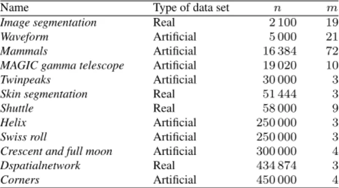
data sets are taken fromMATLAB Central File Exchange. Each data set has some specific characteristics. The short descriptions of the data sets are presented in Table 1.
Table 1.Data sets (n– number of instances,m– number of features).
Name Type of data set n m
Image segmentation Real 2 100 19
Waveform Artificial 5 000 21
Mammals Artificial 16 384 72
MAGIC gamma telescope Artificial 19 020 10
Twinpeaks Artificial 30 000 3
Skin segmentation Real 51 444 3
Shuttle Real 58 000 9
Helix Artificial 250 000 3
Swiss roll Artificial 250 000 3
Crescent and full moon Artificial 300 000 4
Dspatialnetwork Real 434 874 3
A personal computer (Intel i5-3317U CPU 1.7 GHz (Max Turbo 2.6 GHz), with 2 cores and 12 GB of RAM memory) is used for the experimental investigation. The explored ways of the projection error calculation are implemented in MATLAB R2012b. When using a computer with other characteristics, absolute values of the computation time would change, but the same ratio value between different ways would remain, while the accuracy of projections will be the same. It is evident that if a computer with other amount of memory is used, memory resources would run out analyzing larger (or smaller) data sets (depending on the amount of memory). The principal component analysis is used to reduce the dimensionality of the initial data set. The main idea of principal component analysis is to reduce the dimensionality of data by performing a linear transformation and rejecting a part of the components, variances of which are the smallest ones [5]. A detailed and rigorous mathematical derivation of this method can be found in [10].
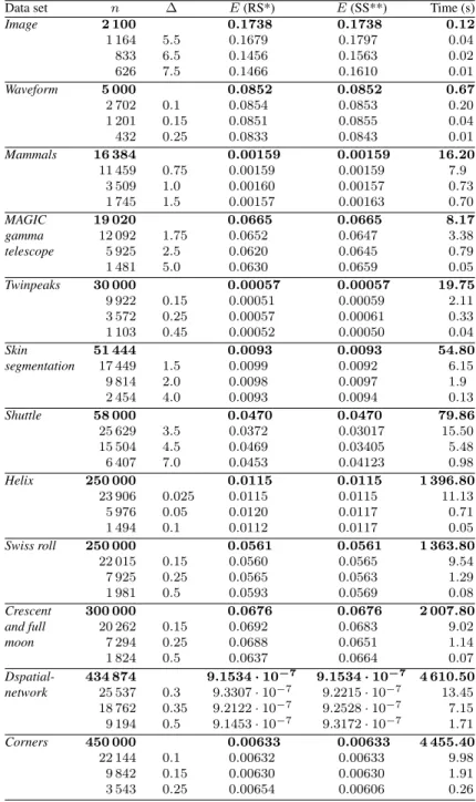
Table 2 shows the results of projecting the data samples of twelve data sets by the principal component analysis when the projection error is calculated for the representative data sample by the proposed first way. Different values of margin of error (∆) and two sampling (random (RS) and stratified (SS)) methods are analyzed. The dimensionality of data is reduced to two (d = 2). The projection error values for the full data sets are also obtained and presented in bold. Some of data sets contained more than 30 000 points therefore the projection error for these data sets was calculated by the proposed second way (see Section 2.2), because other ways are not so efficient (memory shortage or long calculation time) for large data sets. The differences between the projection error values for the data samples of various size and for the full data are not significant when all the data sets are analyzed, even size of representative sample is more less than one of the full data set. From Table 2, one can clearly see that as the margin of error decreases, the data sample size increases. Moreover the difference between stress values of data samples is not essential analyzing all data sets. However the computation time obviously differs, especially for large (containing more than 250 000 points) data sets. For example, the projection error of theCornersdata set is calculated in about 1 hour 14 minutes, that of its random sample (22 144 points) in about 9.98 seconds while the projection error values are 0.0632 and 0.0633, respectively. The comparison of two sampling methods shows that it is unimportant how the sample was obtained, i.e., the projection error values are similar in both cases. For example, the projection error of the fullHelix data set is 0.0115, that of its random sample (1 494 points) is 0.0117, that of the stratified sample (1 494 points) is 0.0112. While analyzing data samples of 23 906 points, the projection error values are the same as for the full data set and for its samples and equal to 0.0115. The visualization of theHelix data set and its data samples, when their dimensionality is reduced by the principal component analysis, is presented in Fig. 1. The images show that the distribution of the points of random and stratified data samples is similar to that of the initial data set. It can be emphasized that the loss of projection error accuracy is not significant compared to the computation time we save. The experimental results show that the projection error can be evaluated for the representative sample when large data sets are analyzed.
Table 3 shows the computation time results of the second way, i.e., the projection error is obtained using the full data set which is divided into the smaller data sets.
Table 2. Projection errorE and computation time values in seconds (s) for twelve different data sets (n– sample size,∆– margin of error).
Data set n ∆ E(RS*) E(SS**) Time (s)
Image 2 100 0.1738 0.1738 0.12 1 164 5.5 0.1679 0.1797 0.04 833 6.5 0.1456 0.1563 0.02 626 7.5 0.1466 0.1610 0.01 Waveform 5 000 0.0852 0.0852 0.67 2 702 0.1 0.0854 0.0853 0.20 1 201 0.15 0.0851 0.0855 0.04 432 0.25 0.0833 0.0843 0.01 Mammals 16 384 0.00159 0.00159 16.20 11 459 0.75 0.00159 0.00159 7.9 3 509 1.0 0.00160 0.00157 0.73 1 745 1.5 0.00157 0.00163 0.70 MAGIC 19 020 0.0665 0.0665 8.17 gamma 12 092 1.75 0.0652 0.0647 3.38 telescope 5 925 2.5 0.0620 0.0645 0.79 1 481 5.0 0.0630 0.0659 0.05 Twinpeaks 30 000 0.00057 0.00057 19.75 9 922 0.15 0.00051 0.00059 2.11 3 572 0.25 0.00057 0.00061 0.33 1 103 0.45 0.00052 0.00050 0.04 Skin 51 444 0.0093 0.0093 54.80 segmentation 17 449 1.5 0.0099 0.0092 6.15 9 814 2.0 0.0098 0.0097 1.9 2 454 4.0 0.0093 0.0094 0.13 Shuttle 58 000 0.0470 0.0470 79.86 25 629 3.5 0.0372 0.03017 15.50 15 504 4.5 0.0469 0.03405 5.48 6 407 7.0 0.0453 0.04123 0.98 Helix 250 000 0.0115 0.0115 1 396.80 23 906 0.025 0.0115 0.0115 11.13 5 976 0.05 0.0120 0.0117 0.71 1 494 0.1 0.0112 0.0117 0.05 Swiss roll 250 000 0.0561 0.0561 1 363.80 22 015 0.15 0.0560 0.0565 9.54 7 925 0.25 0.0565 0.0563 1.29 1 981 0.5 0.0593 0.0569 0.08 Crescent 300 000 0.0676 0.0676 2 007.80 and full 20 262 0.15 0.0692 0.0683 9.02 moon 7 294 0.25 0.0688 0.0651 1.14 1 824 0.5 0.0637 0.0664 0.07 Dspatial- 434 874 9.1534·10−7 9.1534·10−7 4 610.50 network 25 537 0.3 9.3307·10−7 9.2215·10−7 13.45 18 762 0.35 9.2122·10−7 9.2528·10−7 7.15 9 194 0.5 9.1453·10−7 9.3172·10−7 1.71 Corners 450 000 0.00633 0.00633 4 455.40 22 144 0.1 0.00632 0.00633 9.98 9 842 0.15 0.00630 0.00630 1.91 3 543 0.25 0.00654 0.00606 0.26 * – random sampling (RS) ** – startified sampling (SS)
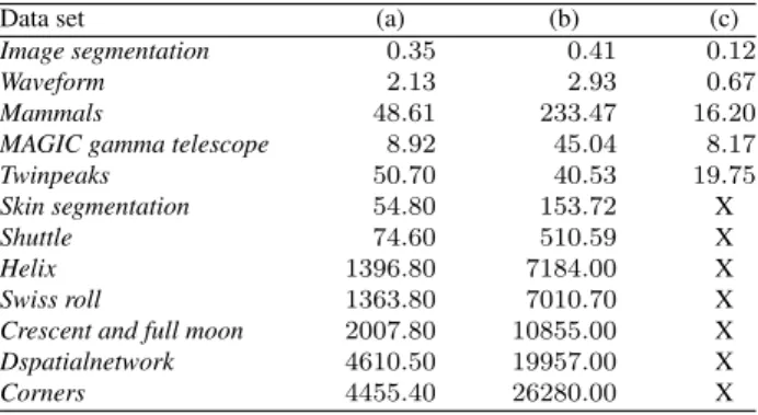
Table 3.Computation time values in seconds (s) of projection error for twelve different data sets: (a) data set is divided (the second way); (b) the loop for each data point is used; (c) distances are found using MATLAB functionpdist.
Data set (a) (b) (c)
Image segmentation 0.35 0.41 0.12
Waveform 2.13 2.93 0.67
Mammals 48.61 233.47 16.20
MAGIC gamma telescope 8.92 45.04 8.17
Twinpeaks 50.70 40.53 19.75
Skin segmentation 54.80 153.72 X
Shuttle 74.60 510.59 X
Helix 1396.80 7184.00 X
Swiss roll 1363.80 7010.70 X
Crescent and full moon 2007.80 10855.00 X
Dspatialnetwork 4610.50 19957.00 X
Corners 4455.40 26280.00 X
X – memory resources run out
Figure 1. Visualization of theHelixdata set and the data samples. Projection error values are shown in the bottom left corner.
Here the data sets are divided into the data sets of the size 10 000 points (for small data sets the size is 500 points). In addition the computation time of projection error, when distances between points are found using thepdistfunction and using the loop for each data point is presented in Table 3. The results have shown that the fastest way to calculate the projection error is to use thepdistfunction for not divided data set or to use thepdist and the pdist2functions for divided data set (the second way). Fast computation time is caused particularity of the MATLAB language which provides native support for the vector and matrix operations, enabling fast development and execution. However using the pdist function for not divided data set causes the computer to run out of memory resources (12 GB) when data sets of more than 30 000 are analyzed. The most time consuming way to calculate the projection error is to use the loop for each data point, but this way does not require much computer memory. The analysis of 450 000 instances has shown that the projection error is calculated in about 7 hours and 18 minutes. So this calculation way is not appropriate for very large data sets. Dividing the data set into the smaller data sets allows us to process the data set of 450 000 instances in an appropriate time (1 hour and 14 minutes).
4
Conclusions
In the paper, we have proposed and explored two ways for projection error evaluation, when large data sets are analyzed using a personal computer without any particular pro-gramming and technologies for high performance computing. The first way calculates the projection error for representative data sample, the second way divides the data set into the smaller data sets.
The experimental investigation with twelve real and artificial data sets has shown that in order to decrease computation time, the projection error can be evaluated precisely using only representative data sample, but not full data set. The differences between the projection error values of the data samples and the full data are not significant analyzing all data sets. Furthermore the projection error calculation for the representative data sam-ple significantly saves computation time. The results have shown that dividing data set into the smaller data sets allows us to calculate the projection error for data of 450 000 instances in an appropriate time and is capable to process larger data sets. Results indicate that the combination of these proposed ways would allow us to calculate the projection error for very large data sets which representative data sample would contain 450 000 points or even more, the projection would be sufficiently precise, the projection error evaluation would be obtained in an appropriate time, and computer memory problem would not arise. The combination could be implemented in this way: first of all, having a large volume data set, the representative data sample should be chosen, and then by dividing the representative data sample into the smaller sets, the projection error could be calculated.
References
1. E.J. Bartlett, J.W. Kotrlik, C.C. Higgins, Organizational research: Determining appropriate sample size in survey research,Information Technology, Learning, and Performance Journal, 19(1):43–50, 2001.
2. E. Bingham, H. Mannila, Random projection in dimensionality reduction: Applications to image and text data, inProceedings of the Seventh ACM SIGKDD International Conference on Knowledge Discovery and Data Mining, ACM Press, New York, 2001, pp. 245–250. 3. I. Borg, P. Groenen, Modern Multidimensional Scaling: Theory and Applications, 2 ed.,
Springer, New York, 2005.
4. N. Choudhary, P. Singh, Cloud computing and big data analytics, International Journal of Engineering Research and Technology,2(12):2700–2704, 2013.
5. G. Dzemyda, O. Kurasova, J. Žilinskas, Multidimensional Data Visualization: Methods and Applications, 1 ed., Springer, New York, 2013.
6. A. Gisbrecht, B. Hammer, Data visualization by nonlinear dimensionality reduction, Data Mining and Knowledge Discovery,5(2):51–73, 2015.
7. A. Gupta, R. Bowden, Evaluating dimensionality reduction techniques for visual category recognition using renyi entropy, in19th European Signal Processing Conference (EUSIPCO 2011), IEEE, Barcelona, 2011, pp. 913–917.
8. J. Han, M. Kamber,Data Mining Concepts and Techniques, 2 ed., Morgan Kaufman Publishers, San Francisco, 2006.
9. P. Joia, F.V. Paulovich, D. Coimbra, J.A. Cuminato, L.G. Nonato, Local affine multidi-mensional projection,IEEE Transactions on Visualization and Computer Graphics, 17(12): 2563–2571, 2011.
10. I. Joliffe,Principle Component Analysis, 2 ed., Springer, New York, 2002.
11. O. Kurasova, A. Molyt˙e, Quality of quantization and visualization of vectors obtained by neural gas and self-organizing map,Informatica,22(1):115–134, 2011.
12. Q. Liu, A.H. Sung, B. Ribeiro, D. Suryakumar, Mining the big data: The critical feature dimension problem, in2014 IIAI 3rd International Conference on Advanced Applied Infor-matics (IIAI-AAI 2014), IEEE, Kitakyushu, 2014, pp. 499–504.
13. V. Medvedev, G. Dzemyda, O. Kurasova, V. Marcinkeviˇcius, Efficient data projection for visual analysis of large data sets using neural networks,Informatica,22(4):507–520, 2011.
14. B. Mwangi, T.S. Tian, J.C. Soares, A review of feature reduction techniques in neuroimaging,
Neuroinformatics,12(2):229–244, 2014.
15. D. O’Leary, Artificial intelligence and big data,IEEE Intelligent Systems,28(2):96–99, 2013. 16. K. Paulauskien˙e, O. Kurasova, Analysis of dimensionality reduction methods for various
volume data, in Information Technology. 19th Interuniversity Conference on Information Society and University Studies (IVUS 2014), Technologija, Kaunas, 2014, pp. 114–121 (in Lithuanian).
17. F.V. Paulovich, C.T. Silva, L.G. Nonato, Two-phase mapping for projecting massive data sets,
IEEE Transactions on Visualization and Computer Graphics,16(6):1281–1290, 2010. 18. C. Sorzano, J. Vargas, A. Pascual-Monato, A survey of dimensionality reduction techniques,
Computing Research Repository, 2014, http://arxiv.org/ftp/arxiv/papers/ 1403/1403.2877.pdf.
19. L.P.J. van der Maaten, E.O. Postma, H.J. van den Herik, Dimensionality reduction: A com-parative review, 2009, http://www.iai.uni-bonn.de/~jz/dimensionality_
reduction_a_comparative_review.pdf.
20. X. Wu, X. Zhu, G. Wu, W. Ding, Data mining with big data,IEEE Transactions on Knowledge and Data Engineering,26(1):97–107, 2014.
21. F. Xie, Y. Fan, M. Zhou, Dimensionality reduction by weighted connections between neighborhoods,Abstract and Applied Analysis,2014:1–5, 2014.