IMPROVEMENT AND IMPLEMENTATION OF ANALOGY BASED METHOD FOR SOFTWARE PROJECT COST ESTIMATION

(1)

ANALOGY BASED METHOD FOR SOFTWARE

PROJECT COST ESTIMATION

LI YAN-FU

(B. Eng), WUHAN UNIVERSITY

A THESIS SUBMITTED

FOR THE DEGREE OF DOCTOR OF PHILOSOPHY

DEPARTMENT OF INDUSTRIAL AND SYSTEMS

ENGINEERING

NATIONAL UNIVERSITY OF SINGAPORE

(2)

First and foremost, I would like to record the deepest gratitude to my advisors, Prof. Xie Min and Prof. Goh Thong Ngee, whose patience, motivation, guidance and supports from the very beginning to the final stage of my PhD life enabled me to complete the research works and this thesis.

Besides my advisors, I would like to thank the professors who taught me lectures and gave me wise advices, the student colleagues who provided me a stimulating and fun environment, the laboratory technicians and secretaries who offered me great assistants in many different ways.

I wish to thank my wife and my best friends in NUS for helping me get through the difficult times, and for all the emotional support, entertainment, and caring they provided.

Last but not the least, I should present my full regards to my parents who bore me, raised me, and loved me.

To them I dedicate this thesis. Yanfu Li

(3)

Cost estimation is an important issue in project management. The effective application of project management methodologies often relies on accurate estimates of project cost. Cost estimation for software project is of particular importance as a large amount of the software projects suffer from serious budget overruns. Aiming at accurate cost estimation, several techniques have been proposed in the past decades. Analogy based estimation, which mimics the process of project managers making decisions and inherits the formal expressions of case based reasoning, is one of the most frequently studied methods.

However, analogy based estimation is often criticized for its relatively poor predictive accuracy, large computational expense, and intolerance to uncertain inputs. To alleviate these drawbacks, this thesis is devoted to improve the analogy based method from three aspects: accuracy, efficiency, and robustness.

A number of journal/conference papers have been published under this objective. The research works that have been done are grouped into four chapters (each chapter is focused on one component of analogy based estimation): chapter 3 summarizes the work on mutual information based feature selection technique for similarity function; chapter 4 presents the research on genetic algorithm based project selection method for historical database; chapter 5 presents the work on non-linear adjustment to solution function; chapter 6 presents the probabilistic model of analogy based estimation with focus on the number of nearest neighbors. The remaining chapters in this thesis, namely chapters 2 and 7, are the literature review and the conclusions and future works.

Research in chapters 3 to 5 aims to enhance analogy based estimation‟s accuracy. For instance, in chapter 5 the adjustment mechanism has been largely improved for a more accurate analogy based method. Efficiency is another important aspect of estimation performance. In chapter 3, our study on refining the historical dataset has achieved a significant reduction of unnecessary projects and therefore improved the efficiency of analogy based method. Moreover, in chapter 6 the study on probabilistic model lead to a more robust and reliable analogy based method tolerable to uncertain inputs. The promising results show that this thesis makes significant contributions to the knowledge of analogy based software cost estimation in both the fields of software engineering and project management.

(8)

Table 2.1: Nu mber of publicat ions in each year fro m 1999 to 2008 ...16

Table 2.2: Su mma ry of d iffe rent similarity functions...40

Table 2.3: Su mma ry of papers investigating different number of nearest neighbors...43

Table 2.4: Su mma ry of publications with different solution functions ...45

Table 3.1: Co mparisons of different feature selection schemes ...77

Table 3.2: Se lected features in three data splits ...78

Table 3.3: Times consumed to optimize feature subset (seconds)...80

Table 3.4: M IABE estimation results on Desharnais Dataset ...82

Table 3.5: Co mparisons with published results ...83

Table 3.6: Co mparisons of different feature selection schemes ...84

Table 3.7: Se lected variables for three splits ...86

Table 3.8: Time needed to optimize feature subset (seconds) ...87

Table 3.9: M IABE estimation results on Maxwell Dataset ...89

Table 3.10: Co mparisons with published results ...89

Table 4.1: Results of FWPSA BE on A lbrecht Dataset ... 109

Table 4.2: The results and comparisons on Albrecht Dataset... 110

Table 4.3: Results of FWPSA BE on Desharnais Dataset ... 112

Table 4.4: The results and comparisons on Desharnais Dataset ... 112

Table 4.5: The part ition of a rtific ial data sets... 119

(9)

Table 5.1: Co mparison of published adjustment mechanisms ... 127

Table 5.2: Results of NA BE on Alb recht dataset ... 147

Table 5.3: Accuracy comparison on Albrecht dataset... 148

Table 5.4: NA BE vs. other methods: p-values of the Wilco xon tests and the improvements in percentages... 149

Table 5.5: Results of NA BE on Desharnais dataset... 150

Table 5.6: Accuracy comparisons on Desharnais dataset... 151

Table 5.7: NA BE vs. other methods: p-values of the Wilco xon tests and the improvements in percentages... 152

Table 5.8: Results of NA BE on Ma xwe ll dataset... 153

Table 5.9: Accuracy comparisons on Maxwell dataset... 154

Table 5.10: NA BE vs. other methods: p-values of the Wilco xon tests and the improve ments in percentages... 155

Table 5.11: Results of NABE on ISBSG dataset ... 156

Table 5.12: Accuracy co mparisons on ISBSG dataset... 156

Table 5.13: NA BE vs. other methods: p-values of the Wilco xon tests and the improve ments in percentages... 158

Table 5.14: Characteristics of the four real world datasets ... 159

Table 5.15: Art ific ial datasets and properties ... 163

Table 5.16: Co mparative performance of NA BE to other methods ... 164

Table 5.17: Testing MMREs under diffe rent dataset size ... 165

Table 5.18: Mann-Whitney U tests of dataset size influences ... 166

Table 5.19: Testing MMREs under diffe rent proportions of categorical features ... 167

Table 5.20: Wilco xon tests of proportion of categorical features influences... 168

(10)

Table 6.1: Corre lations between CHANGE and OO metrics ... 187

Table 6.2: Point predict ion accuracy on UIMS dataset ... 192

Table 6.3: Wilco xon signed-rank test on UIMS dataset ... 194

Table 6.4: Results of interval prediction at 95% confidence leve l ... 195

Table 6.5: Point predict ion accuracy on QUES dataset... 196

Table 6.6: Wilco xon signed-rank test on QUES dataset ... 197

(11)

List of Figures

Figure 1.1: The A BE system structure ...6

Figure 1.2: The distribution of research wo rks ...9

Figure 2.1: The classificat ion of software cost estimation methods ...16

Figure 2.2: The distribution of publicat ions of each class during 1999 - 2008...18

Figure 2.3: Rayle igh function in SLIM model...26

Figure 2.4: An e xa mp le of art ificia l neura l network ...35

Figure 3.1: The re lations between mutual informat ion and the entropy...66

Figure 3.2: The schematic d iagra m o f proposed MIABE a lgorithm...69

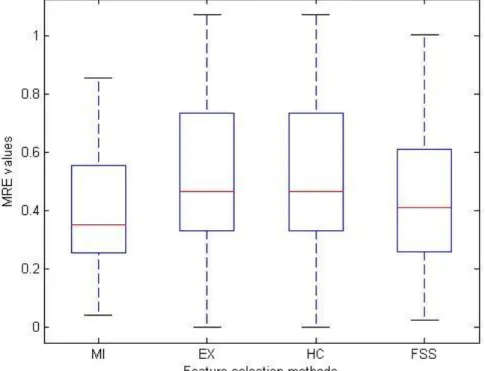
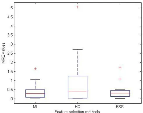
Figure 3.3: The bo xplots of MRE values of feature selection methods ...78

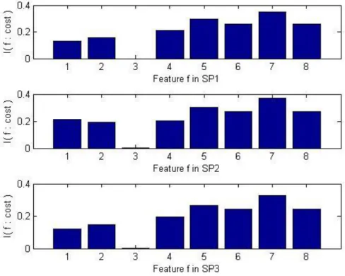
Figure 3.4: Mutual in formation diagra m for the features in three tra ining data splits ...80

Figure 3.5: The bo xplots of MRE values of feature selection methods (EX is not applicable ) 85 Figure 3.6: Mutual in formation diagra m for the features in tra ining dataset ...87

Figure 4.1: Chro mosome for FWPSABE ...97

Figure 4.2: The train ing stage of FWPSABE... 101

Figure 4.3: The testing stage of FWPSABE... 103

Figure 4.4: The testing results on Albrecht Dataset ... 110

Figure 4.5: The testing results on Desharnais Dataset... 113

Figure 4.6: Cost versus size of Albrecht dataset... 115

(12)

Figure 4.9: Y versus x1sk of severe non-Norma lity Data set ... 118

Figure 4.10: The testing results on Artific ial Moderate non -Normality Dataset ... 120

Figure 4.11: The testing results on Artificia l Severe non -Norma lity Dataset... 122

Figure 5.1: The general fra me work of analogy based estimation with adjustment ... 126

Figure 5.2: Train ing stage of the ANN adjusted ABE system with K nearest neighbors ... 136

Figure 5.3: Predicting stage of the ANN ad justed ABE system with K nearest neighbors ... 138

Figure 5.4: Bo xplots of absolute residuals on Albrecht dataset ... 149

Figure 5.5: Bo xplots of absolute residuals on Desharnais dataset ... 152

Figure 5.6: Bo xplots of absolute residuals on Maxwe ll dataset ... 155

Figure 5.7: Bo xplots of absolute residuals on ISBSG dataset... 157

Figure 6.1: Bo xplots of Absolute residuals and MREs on UIMS dataset ... 193

Figure 6.2: Confidence zones on UIMS dataset ... 195

Figure 6.3: Bo xplots of Absolute residuals and MREs on QUES dataset... 197

(13)

List of Abbreviations

ABE: Analogy based estimation ANN: Artificial neural network

BABE: Bootstrapped analogy based estimation CART: Classif ication and regression trees CASE: Computer-aided software engineering

FWABE: Feature weighting for analogy based estimation

FWPSABE: Simultaneous feature weighting and project selection for analogy based estimation

GABE: Genetic algorithm optimized linear function adjusted analogy based estimation

KNNR: K-nearest neighbor regression

LABE: Linear function adjusted analogy based estimation MdMRE: Median Magnitude of Relative Error

MIABE: Mutual information based features selection for analogy based estimation

MMRE: Mean magnitude of relative error MRE: Magnitude of relative error

NABE: Non-linear function adjusted analogy based estimation PABE: Probabilistic model of analogy based estimation PRED(0.25): Prediction at level 0.25

PSABE: Project selection for analogy based estimation

RABE: „Regression toward the mean‟ adjusted analogy based estimation RBF: Radial basis function networks

SABE: Similarity function adjusted analogy based estimation OLS: Ordinary least square regression

SVR: Support vector regression SWR: Stepwise regression

(14)

Chapter 1

Introduction

Recently, the software industry has faced a dramatic increase in the demand of new software products. O n the other hand, software became more and more complex and difficult to produce and maintain. This demand-supply contradiction has contributed to the continuous improvements on software project management in which the ultimate goal is producing low cost and high quality software in short time. Successful software project management requires effective planning and scheduling supported by a group of activities, among which estimating the development cost (or effort) is fundamental to guide other activities. This task is known as Software Cost Estimation. Software cost estimation is a very active research field as it was more than 30 years ago, when the difficulties of estimation were discussed in “The Mythical Man Month” (Brooks 1975).

1.1

Software Cost Estimation

Cost estimation is a critical issue in project management (Chen 2007, Henry et al. 2007, Pollack-Johnson and Liberatore 2006). It is particularly important for software projects, as numerous software projects suffer from overruns (Standing 2004) and accurate cost estimation is one of the key points to the success of software project management.

(15)

Software cost (or effort) estimation is the process of predicting the amount of effort required to build a software system (Boehm 1981). It is a continuous activity which can or must start at the early stage of the software life cycle and continues throughout the life time. During the first phases of software life cycle, cost estimation is of necessity for software developing team to decide whether or not to proceed, though accurate estimates are obtained with great difficulties at this point due to the wrong assumptions or imprecise data. During the middle phases, the cost estimates are useful for rough validation and process monitoring. After completion, cost estimates are useful for project productivity assessment.

Since the software cost estimation affects almost all aspects of software project development such as bidding, budgeting, planning and risk analysis. The estimation has great impacts on software project management. If the estimation is too low, then the software development will be running under considerable constraints to finish the product in time, and the resulting software may not be fully functional or tested. On the other hand, if the estimation is too high, then too many resources will be committed to the project and this may result in significant amount of wasted resources. Furthermore, if the company is engaged in a contract, then too high an estimate may lead to loss of business opportunity.

Despite its importance, the estimation of software cost is still a weakness in software project management. Aiming at accurate and robust estimation,

(16)

various cost estimation techniques have been proposed in past decades. Section 1.2 presents a brief introduction to these techniques including our research focus: analogy based estimation.

1.2

Introduction to Cost Estimation Methods

According to Angelis and Stamelos (2000)‟s classification system, cost estimation methods can be grouped under three categories: expert judgment, algorithmic estimation, and analogy based estimation.

1.2.1 Expert Judgment Based Estimation

Expert judgment requires the consultation of one or more expert s to derive the cost estimate (Hughes 1996). A Dutch study carried out by Heemstra (1992) revealed that 62% of estimators/organizations use this intuition technique and a study carried out later by Vigder and Kark (1994) also confirmed the widespread use of this technique. Despite its popularity this method seems to have received a poor reputation and it is often regarded as subjective and unstructured which makes it vulnerable compared with more structured methods (Angelis and Stamelos 2000).

1.2.2 Algorithmic Based Estimation

To date, the algorithmic method is the most popular technique in the literature. In algorithmic method, cost value is estimated by using certain

(17)

mathematical function to link it to the inputs metrics such as „line of source code‟ and „function points‟. The mathematical model is often built upon some information abstracted from historical projects. Algorithmic method has some advantages over expert judgment: it has well defined formal structure; it produces identical outputs given the same inputs; it is efficient and good for sensitivity analysis (Selby and Boehm 2007).

The algorithmic method consists of a large number of techniques which can be further divided into two classes: function based methods and machine learning methods. Examples of function based methods are: COCOMO model (Boehm 1981), Function Points Analysis (Albrecht and Gaffney 1983), SLIM model (Putnam 1978), and Regressions (Schroeder et al. 1986). Examples of machine learning methods are: Artificial Neural Networks (Srinivasan and Fisher 1995), Classification and Regression Trees (CART) (Brieman et al. 1984).

1.2.3 Analogy Based Estimation

Analogy based estimation (Shepperd and Schofield 1997) is the process of identifying one or more historical projects that are similar to t he project being developed and deriving the estimates from the similar historical projects. This technique is intended to mimic the process of an expert making decisions based on his/her experience. On the other hand, analogy based estimation has a concrete and well-defined estimation framework, given that similar past

(18)

projects can be easily retrieved and the mechanism applying the nearest neighbors is correct. Thus, analogy based estimation is a very flexible method which allows the combination of the good aspects in both algorithmic methods and expert judgment. It has several advantages such as: it is able to deal with poorly understood domains, its output is relatively easy to interpret, and it offers the chance to learn from past experiences (Walkerden and Jeffery 1999).

1.3

Motivations

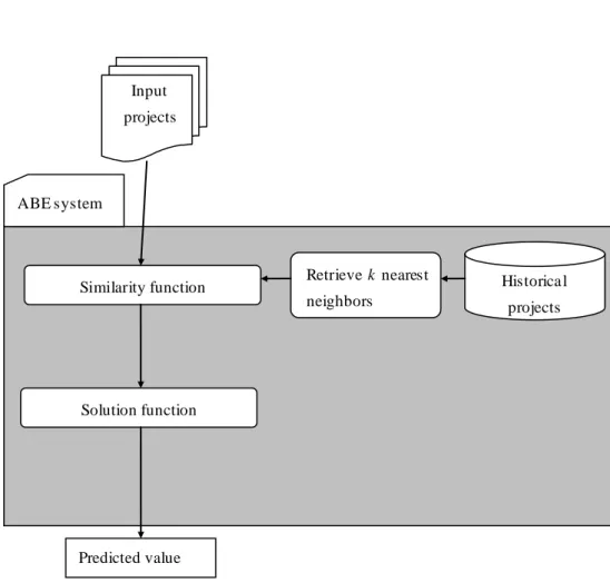
As explained in the previous section, analogy based estimation is one successful technique for cost estimation. However, it also has been criticized for relatively poor predictive accuracy, large computational expense, and intolerance to uncertainties. To overcome these drawbacks, many research works have been focusing on improving the four key components of analogy based system: similarity function, historical database, number of retrieved nearest neighbors and solution function (shown in Fig 1.1).

Similarity function (Shepperd and Schofield 1997), which measures the level of similarity between two different projects, is one of the key components in analogy based system. The choice of measure is an important issue since it affects the projects to be selected as the nearest neighbors. Many works (Auer et al., 2006, Huang and Chiu, 2006, Mendes et al., 2003) have been devoted to optimize the similarity function or feature weights, and the

(19)

prediction accuracy of the analogy based system was reported to be significantly improved if the appropriate similarity functions or feature weights have been selected.

The historical database is the storage of the past projects‟ information, and it is used to retrieve the nearest neighbors. However, due to the instability of software development process the historical databases always contain noisy or redundant projects which might ultimately hinder the prediction accuracy of analogy based estimation. One possible solution is to reduce the whole database into smaller subset that consists of merely the representative projects.

Similarity function Input projects Predicted value Historica l projects Solution function Retrieve k nearest neighbors ABE system

(20)

Despite the importance of subset selection, very few research works (Kirsopp and Shepperd 2002) have been focused on this topic.

The number K of retrieved nearest neighbors decides how many nearest neighbors should be selected for the solution function to generate final prediction. Many works (Li and Ruhe. 2008, Mittas et al. 2008, Auer et al. 2006, Mendes et al. 2003, Leung 2002) have investigated the impacts of this value on the estimation results and/or considered optimiz ing this value. However, to our knowledge there is no widely accepted technique to choose K except the empirical trial-and-error method. Therefore, it is of great interest to develop systematic ways to optimize this parameter.

The solution function calculates the final estimation results from the nearest neighbors retrieved from the historical database. If an appropriate solution function is used, the prediction performance of analogy based system could be improved significantly. In the literature, only linear solution functions (Chiu and Huang, 2007, Jorgensen et al., 2003) have been considered though the relationships between the cost value and input features are usually non- linear. There is still a lack of research works to investigate the feasibility of applying non- linear solution functions.

As discussed above, many studies have been devoted to achieve accurate prediction by improving the four components of the analogy based system; however there still exists great opportunities to improve analogy based estimation for better performance. Moreover, most of the previous studies

(21)

merely focused on improving accuracy which is one aspect of performance. The robustness, which is another important indicator, has received few concerns. As budget uncertainty is an important issue in project management (Yang 2005, Barraza and Bueno 2007), some authors pointed out that it is safer to generate probabilistic predictions such as probability distributions o f the effort values or interval estimates with a probability. However, very little research (Angelis and Stamelos 2000, Jorgensen and Sjoberg 2003, van Koten and Gray 2006) has been done on probabilistic predictions.

1.4

Research Objective

The objective of this thesis is to improve accuracy, efficiency and robustness of analogy based estimation. Accuracy is the indicator of the cost estimator‟s ability to produce the quality predictions that match the software projects‟ costs. Efficiency is the speed of the cost estimator to complete a certain amount of estimation tasks. Robustness reflects the cost estimator‟s tolerance to uncertain inputs such as missing values and noisy data.

A number of journal/conference papers have been published under this objective. The research works that have been done are grouped into four chapters (each chapter is focused on one component of analogy based estimation): chapter 3 summarizes the works on mutual information based feature selection technique for similarity function; chapter 4 presents the research on genetic algorithm based project selection method for historical

(22)

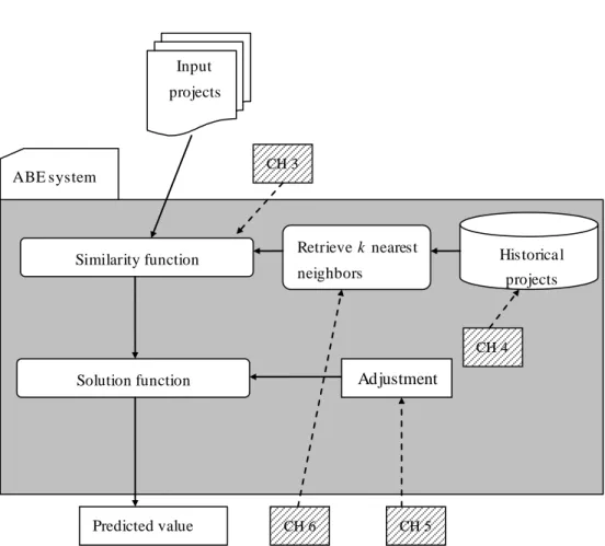
database; chapter 5 presents the work on non-linear adjustment to solution function; chapter 6 presents the probabilistic model of analogy based estimation which is focused on the number of nearest neighbors. The distribution of chapters 3 to 6 in the framework of analogy based system is illustrated in fig 1.2 where the shaded boxes with characters „CH‟ stand for chapters (e.g. CH 3 stands for chapter 3). The remaining chapters in this thesis, namely chapters 2 and 7, are the literature review and the conclusions.

All of our research works share a common objective - enhance the analogy based estimation‟s capability to achieve more accurate results. In

Similarity function Input projects Predicted value Historica l projects Solution function CH 4 CH 5 CH 6 Retrieve k nearest neighbors CH 3 ABE system Adjustment

(23)

practice, this is very important for the software enterprises to maintain a better control of the budget throughout their software development processes. Theoretically speaking, these studies have contributed to the optimization of individual component of analogy based system. For instance, historical database and solution function have been largely refined or improved in our works. Furthermore, these studies point out a feasible direction to the global optimization of analogy based system.

Efficiency is another important aspect of estimation performance. In practice, improving estimation efficiency means enhanc ing the chance of winning bids. Many machine learning methods such as ANN and RBF can be very accurate in some situations, but they are often suffering from slow training speed. In addition, expert judgment could also be time consuming, as it usually takes time to gather/interview experts. Our studies on refining the historical dataset of analogy based system have achieved a significant reduction of unnecessary projects. Consequently, the efficienc y of analogy based system is largely improved by our algorithm.

Moreover, the studies on probabilistic model lead to a more robust and reliable analogy based system. These studies could enhance the system‟s capability to deal with a broader scope of situations such as missing values and ambiguous inputs. Additionally, the probabilistic prediction provides a feasible way to model the inherited uncertainties and variabilities in the software development process.

(24)

As mentioned above, our research on analogy based estimation is of significant theoretical value and practical value. For a better understanding of our research work, the detailed background information of our research work is presented in the literature review in next chapter.

(25)

Chapter 2

Literature

Review on Software Cost

Estimation Methods

To obtain accurate software project cost estimates, various kinds of methods have been proposed. This chapter provides a detailed summary of the software cost estimation methods published in the past decade. The evaluation criteria for the prediction accuracy of these methods are also summarized and analyzed.

2.1

Introduction

In the literature there are several comprehensive overviews on the cost estimation methods, such as Walkerden and Jeffery (1997), Boehm et al. (2000), Briand and Wieczorek (2002), Jorgensen (2004a) and Jorgensen and Shepperd (2007). Among them, some reviews (Walkerden and Jeffery 1997, Boehm et al. 2000, Briand and Wieczorek 2002) have proposed different classification systems.

Walkerden and Jeffery (1997) introduced a system with four classes of estimation methods: empirical, analogical, theoretical, and heuristic. However, they stated that expert judgment cannot be included into their system. Moreover, there are overlaps between analogical and empirical, as analogical

(26)

estimation process often involves empirical decisions (such as the choice of similarity measures in analogy based method) (Briand and Wieczorek 2002). Lately, Briand and Wieczorek (2002) defined a hierarchical scheme starting from two major classes (model-based methods, non- model-based methods) that are further divided into several sub-classes. The sub-classes contain further divisions and so on. Although the authors claimed that their system covers most types of estimation methods, the hierarchical system has a more complicated tree type structure with more intermediate nodes than other flatter systems and each intermediate node needs its own definition (such as „data driven‟ and „proprietary‟). Boehm et al. (2000) proposed a simpler but comprehensive framework consisting of six major classes: parametric models, expert judgment, learning oriented techniques, regression based methods, dynamic based models, and composite methods. Directly under each major class are the estimation methods and this system can include most types of estimation methods (Boehm et al. 2000). Our classification system is modified from Boehm‟s framework with the consideration to balance the number of recent publications under each major class.

2.2

Literature Survey and Classification System

Prior to our classification system, a structured literature survey is conducted to select the related journal papers during the period between 1999 and 2008. The keywords used for searches in SCI engine are „software cost

(27)

estimation‟, „software effort estimation‟, „software resource estimation‟, „software effort prediction‟, „software cost prediction‟, „software resource prediction‟, and „software prediction‟. The main criterion for including a journal paper in the survey is that the paper presents research on software development effort or cost estimation. Papers related to prediction of software size/defects, modeling of software process, or identification of factors correlated with software project cost, are included only if the main purpose of the study is to improve software cost estimation. The papers with pure discussions or opinions are excluded. The process above results in a collection of 158 journal papers.

To construct our classification system, we first calculate the number of publications under each category in Boehm (2000)‟s system. The results reveal that the recent research trend has different emphases on each category, for example there are more than 80 papers related to „learning oriented techniques‟ while only 5 papers and 4 papers under „dynamic based models‟ and „composite methods‟ respectively. In addition, Boehm‟s scheme does not include the discrete event simulation model which has only recently appeared as one promising technique. Moreover, there are 35 papers related to „analogy based estimation‟ which stands for the largest proportion among the „learning oriented techniques‟.

For a more balanced structure, we combine the classes „dynamic based models‟, „composite methods‟ and other emerging methods (such as discrete

(28)

event simulation) to form the category „Other methods‟. Furthermore, we split the „analogy based estimation‟ from the „learning oriented techniques‟ to be a major class, and we rename the remaining methods under „learning oriented techniques‟ as „machine learning techniques‟. The reason for this splitting is that analogy based method is the learning oriented method with highest amount of publications and many previous studies (Walkerden and Jeffery 1997, Angelis and Stamelos 2000) have already regarded it as one major class. Analogy based estimation is particularly popular in the context of software cost estimation which might be due to the fact that analogy based estimation build up the connections between project managers making cost estimation based on the memories of past experiences and the formal use of analogies in Case Based Reasoning (CBR) (Kolodner 1993).

From the discussion above, our classification system is established in Fig 2.1. It contains six major categories: expert judgment, parametric models, regressions, machine learning methods, analogy based estimation, and other methods.

Based on our classification system, the number of publications per year of each major class is summarized in table 2.1. It is seen that regressions and machine learning methods are the most popular methods in the past decade. Parametric models and analogy based estimation rank at the third place.

(29)

COCOM O: constructive cost model, FPM : Function point model, SLIM : software life-cycle model, ANN: artificial neural networks, BM : Bayesian methods, CART: classification and regression trees, RBF: radial basis functions, SVM : support vector machine, GP: genetic programming, FL: fuzzy logic, OLS: ordinary least-square regression, RR: robust regression, SWR: stepwise regression, DM : dynamics models, CM : composite methods, SM : simulation models.

Table 2.1: Nu mber of publicat ions in each year fro m 1999 to 2008

Yea r EJ PM RE ML AB OT 1999 2 3 4 1 1 1 2000 1 2 5 5 3 1 2001 3 4 8 6 5 3 2002 0 4 4 4 1 1 2003 4 2 6 5 6 2 2004 7 1 3 3 1 2 2005 3 3 6 6 1 1 2006 2 6 5 8 3 4 2007 3 6 8 5 5 3 2008 3 4 10 10 9 2 Total 28 35 59 53 35 20

EJ: expert judgment, PM : parametric models, RE: regressions Estimation methods Expert judgment M achine learning Parametric models Analogy based estimation COCOM O Regressions FPM SLIM Other method s OLS RR SWR DM CM ANN BM CART RBF SVM GP FL SM

(30)

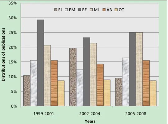
To investigate the trends of publications, the proportion of each class from 1999 to 2008 is depicted in the bar-charts of fig 2.2. The whole period is divided into three nearly equal segments: 1999 – 2001, 2002 – 2004, and 2005 – 2008. Fig 2.2 suggests that:

 Regression technique is the most frequently used method. This observation confirms with Jorgensen and Shepperd (2007)‟s survey. Among the regression papers, a large number of papers use regressions to compare with the estimation methods they propose.

 The proportion of papers on machine learning methods is constantly increasing and they have the same proportion of publications as regressions have in recent 4 years. Unlike regression papers, majority of machine learning papers introduce or propose new cost estimation techniques.

 The proportions of papers on parametric models and analogy based estimation are around 15% with some small fluctuations.

 The popularity of expert judgment based estimation was at its highest in the period 2002-2004.

 The proportion of „other methods‟ is around 8% throughout the past decade.

 The distributions of the papers become more and more even, as in the period after 2001 no method stands for a proportion larger than 25%. This observation is one supportive evidence for our modifications to Boehm‟s classification system.

In the following sections, a comprehensive review is presented for each major class.

(31)

Figure 2.2: The distribution of publicat ions of each class during 1999 - 2008

EJ: expert judgment, PM: parametric models, RE: regressions, ML: machine learning methods, AB: analogy based estimation, OT: other methods

2.3

Cost Estimation Methods

2.3.1 Expert Judgment

Expert judgment requires the consultation of one or more experts to derive the cost estimate (Hughes 1996). With their experience and understanding of the new project and the experience from past projects, the experts could obtain the estimation by a non-explicit and non-recoverable reasoning process, i.e., “intuition”. As reported in the business forecasting study conducted by Blattberg and Hoch (1990), most estimation processes have both intuitive and explicit reasoning elements. In fact, even formal software cost estimation models may require expert estimates as important input parameters (Pengelly,

0% 5% 10% 15% 20% 25% 30% 35% 1999-2001 2002-2004 2005-2008 D is tr ibut ions of pub lic at ions Years EJ PM RE ML AB OT

(32)

1995). Jorgensen (2004a) presented an extensive review of studies related to the expert estimations conducted before 2003. As a subsequent work of Jorgensen (2004a)‟s, we focus on the expert judgment studies published after 2003. Expert judgment often encounters a number of issues, such as estimate uncertainty, bias caused by over-optimism, and etc. A number of research works are aiming to solve these problems.

To describe the uncertainty of cost estimate, Jorgensen and Sjoberg (2003) proposed and evaluated a Prediction Interval (PI) approach, which is based on the assumption that the estimation accuracy of earlier so ftware project predicts the cost PIs of new projects. Lately, Jorgensen et al. (2004) conducted four studies on expert judgment based PIs. The results suggest that the PIs were generally much too narrow to reflect the chosen level of confidence. Moreover, Jorgensen (2004b) claimed that the traditional request for PIs is not optimal and leads to overoptimistic views about the level of estimation uncertainty.

Many works are devoted to the study of the over-optimism phenomenon. Moløkken and Jørgensen (2005) observed that people with technical competence provided more overoptimistic estimates than those with less technical competence. Jørgensen et al. (2006) examined the degree to which level of optimism in software engineers‟ predictions is related to optimism on previous predictions. Jørgensen et al. (2007) concluded that optimistic software engineers have a number of characteristics such as higher confidence in their own predictions, lower development skills, poorer ability or

(33)

willingness to recall effort on previous tasks, and etc. Some techniques are proposed to reduce the bias towards over-optimism. Jorgensen (2005) provided some evidence based guidelines for assessing the uncertainties in expert judgment. Moløkken and Jørgensen (2004) propose an approach combining the judgments of experts with different backgrounds by means of group discussion.

In addition, other studies summarize different characteristics of expert judgment. Jorgensen and Sjoberg (2004) discovery that customer expectations of a project's total cost can have a very large impact on expert judgment. McDonald (2005) shows that cost estimates are dependent upon two kinds of team experience: (1) the average experience for the members of each team and (2) whether or not any members of the team have similar project experience. Grimstad and Jørgensen (2007) reported a high degree of inconsistency in the previous experts‟ estimates. Jorgensen (2004d) suggested that the recall of very similar previously completed projects seemed to be a pre-condition for accurate top-down based estimates.

Although expert judgment has been used widely, the estimates are obtained in a way that is not explicit and consequently difficult to be repeated. Nevertheless, expert judgment can be an effective estimate tool when used as an adjustment factor for algorithmic models (Gray et al. 1999).

(34)

2.3.2 Parametric Models

Parametric models are defined by mathematical formula and need to be calibrated to local circumstances in order to establish the relationship between the cost and one or more project features (cost drivers). Usually, the principal cost driver used in such models is software size (for instance, lines of source code, the number of function points, pages, etc.). This section includes three function methods, COCOMO (Boehm, 1981), Function Points Analysis (Albrecht and Gaffney, 1983), and SLIM model (Putnam, 1978).

COCOMO (Constructive Cost Model)

COCOMO I is one of the best known and best documented software cost estimation model (Boehm 1981). It is a set of three modeling levels: basic, intermediate, and detailed. The basic COCOMO takes the following relationship between cost (effort) and size:

b

KLOC a

Y  ( ) _(2.1)

where Y is the project effort/cost, KLOC represents the size in terms of thousands of lines of source code, and the coefficients a and b depend on COCOMO‟s modeling level and the mode of the project to be estimated (organic, semidetached, embedded). In all cases, the value of b is greater than 1. The intermediate and detailed COCOMO takes the following general form:

(35)

i i b EM KLOC a Y 15 1 ) (    (2.2)

where EMi is the ith effort multiplier. Effort multiplier is the parameter

that affects effort the same degree regardless of project size. However, COCOMO together with its Ada (Kaplan 1991) update are prone to difficulties in estimating the costs of software developed in new lifecycle processes and capabilities (such as iterative model and spiral model).

The research on COCOMO II started in 1994. COCOMO II (Boehm et al. 1995) has two models (early design and post architecture) for cost estimation at different development stages. Early design model is used in the initial stages of a software project when very little information is known about the product being developed. The post architecture model is the most detailed estimation model and it is used when software lifecycle architecture has been developed. The early design and post architecture models share a common form:



      5 1 1 ) ( 01 . 0 01 . 1 ) ( j j i n i b factor scale b EM KLOC a Y (2.3)

where the five „scale factors‟ are the parameters that have large influence on big projects and small influence on small projects (which is different from

(36)

the effort multipliers). The scale factors are precedentedness, development flexibility, risk resolution, team cohesion, and process maturity. Early design model and post architecture model have different number (n) of effort multipliers. Detailed descriptions about the effort multipliers can be found in (Boehm et al. 1995)

Lately, a lot of research works have been done on the COCOMO models. Chulani et al. (1998) proposed a new version of COCOMO II model which includes a 10% weighted average approach to adjust prior expert determined model parameters. Moreover, Chulani et al. (1999) introduced the Bayesian inference for the tuning of the expert determined model parameters. Jongmoon et al. (2002) proposed a way of integrating CASE tool into COCOMO II and their approach resulted in an increase in the prediction accuracy. Benediktsson et al. (2003) introduced the COCOMO-style cost model for the incremental development and explore the relationship between effort and the number of increments. Han et al. (2005) adopted COCOMO model for software project financial budget optimization. Huang et al. (2007) proposed a novel neuro-fuzzy COCOMO model and the authors report that this model greatly improves estimation accuracy. More recently, Fairley (2007) provided a comprehensive overview on COCOMO models. This paper presents a summary of recent work on COCOMO modeling and provides future directions for COCOMO-based education and training.

(37)

Function Points Model (FPM)

The function point (FP) measure was first developed by Albrecht (1979) as an alternative to lines of code for measuring the software size. The function point method defines five basic function types to estimate the size of the software. The five functions types are internal logical files (ILF), external interface files (EIF), external inputs (EI), external outputs (EO), and external inquiries (EQ).

Based on the definition of function points, a number of researchers (Albrecht and Gaffney 1983, Kemerer 1987, Matson et al. 1994, Abran and Robillard 1996) used FP for cost estimation. In their studies, each function point is first classified into one of three complexity levels: low, average or high. Then an integer complexity value is assigned to the function point based on the ordinal scale complexity classification. Furthermore all the identified function complexity values are added together to derive an unadjusted function point count (FPC). Additionally, this count is often adjusted by up to 14 technical complexity factors that account for a variety of non- functional system requirements (e.g. performance, reliability, backup and recovery etc.) to give an adjusted function point count (AFPC). The resulting counts are then used to derive the cost estimate by using the following form:

) (AFPC FPC b a Y    (2.4)

(38)

where a and b are the coefficients determined by ordinary linear regression method. As the software industry keeps evolving rapidly, many other types of size metrics are developed, such as Weighted Methods per Class (WMC), Number Of Children (NOC) (Chidamber and Kemerer 1994), and Class Point (CP) (Costagliola et al. 2005). However, many current papers still considered function point as one of the critical factors in their cost models (Kitchenham et al. 2002, Ahn et al 2003, Moses and Farrow 2005).

Software Life-cycle Model (SLIM)

Putnam (1992) first developed the Software Life-cycle Model (SLIM). The basic assumption of SLIM is that the Rayleigh distribution (See Fig 2.3) can be used to model the change of staff levels on large software projects which have more than 70,000 „Thousands of Delivered Source Instruction‟s (KDSI). It is assumed that the number of people working on a project is a function of time. A project starts with relatively few people and the manpower reaches a peak and then falls off. The decrease in manpower during the testing is less than that during the earlier construction phase. In addition, Putnam explicitly excluded requirements analysis and feasibility studies from the life cycle.

The basic Rayleigh curve (Fig 2.3) defining the effort distribution is described by the following differential equation:

(39)

) exp( 2Kat at2 dt dy   (2.5)

where t is elapsed time from the starting point of a software project, K is the total project effort, and a is a constant that determines the shape of the curve.

Figure 2.3: Rayle igh function in SLIM model

In order to obtain the total project effort K and development time td, the

following two formulas can be derived after a few algebraic manipulations:

7 4 0 7 9 7 1 3 0 3 D C S K C D S t_d               (2.6)

where S is the system size measured by KDSI (Thousands of Delivered Source Instructions), D0 is the manpower acceleration, and C is the

Staff Level

(40)

technology factor. SLIM does not gain much popularity as COCOMO and FPM. However, in the early 2000‟s the company named „Quantitative Software Management‟ has developed a successful package of three tools based on Putnam‟s SLIM. These include SLIM-Estimate, SLIM-Control and SLIMMetrics. SLIM-Estimate is a project planning tool, SLIM-Control is a project tracking and oversight tool, and SLIM-Metrics is a software metrics repository and benchmarking tool. More information on these SLIM tools can be found at http://www.qsm.com.

2.3.3 Regressions

According to our survey, regression methods are most popular in the past decade. The most commonly used regressions method is the Ordinary Least Square (OLS) regression which has also been criticized for its restrictive assumptions and poor performance. This section also includes other types of regression such as robust regression and stepwise regression. These techniques are regarded as the improved version of OLS regression.

Ordinary least-square regression (OLS regression)

OLS regression is one of the most commonly used models for cost estimation. In general, a linear regression has the following form:

e X b X b X b a Yˆ   ₁ ₁ ₂ ₂... _n _n (2.7)

(41)

where Yˆ denotes the dependent variable (project cost/effort), Xi stands for

independent variables (project features/cost drivers), and bi is the so called

regression coefficient, a is referred as the intercept, and the error term e is a random noise with a normal distribution.

The OLS regression has a number of strong assumptions. One important assumption is the so called homoscedasticity which means that the differences between the actual values and the predicted values do not change under different values of Xi. Another assumption is that OLS variables are all

continuous in nature. Thirdly, OLS regression requires that there are no outlier values in both independent and dependent variables. However, extreme outliers are commonly found in software engineering dataset, probably due to the misunderstandings or lack of precision in the data collection process. Finally, no missing data is allowed in OLS regression. On the contrary, missing data is often reported when there is limited time and budget for data collection. In all, many of the difficulties discussed above can be solved by some advanced techniques such as robust regression, logistic regression and data imputation. However these advanced techniques remain difficult to be implemented by most engineers and managers, and applying them still requires extensive training and experience (Briand and Wieczorek 2002).

Although OLS regression is one of the oldest methods for cost estimation, it is still widely applied and continuously improved for more accurate

(42)

predictions. Kitchenham (1998) proposed analysis of variance (ANOVA) and OLS regression to analyze unbalanced data sets. Angelis et al. (2001) proposed categorical regression (CATREG) for the datasets with large number of categorical attributes, such as ISBSG (ISBSG, 2007) dataset. Sentas et al. (2005) modified the standard OLS regression to produce the interval predictions. Jeffery et al. (2000) applied OLS regression on both ISBSG data and company specific data with comparison against analogy based method. More recently, Jorgensen (2004) conducted some regression analysis of cost estimation on a data collection of 49 software development projects. Lucia et al. (2005) applied multivariate OLS regression for corrective maintenance effort estimation. Mendes et al. (2005) applied multivariate OLS regression for Web effort estimation. Multivariate OLS has identified „total number of Web pages‟ and „features provided by the application‟ to be the two most influential effort predictors. Costagliola et al. (2005) applied multivariate OLS regression to predict development effort of object oriented systems by using class points.

Robust Regressions (RR)

Robust regressions are an improved version of OLS regression. They alleviate OLS regression‟s sensitivity to outliers. Instead of minimizing the sum of square of absolute error in OLS regression, robust regressions use other objectives for optimization. There are several types robust regression

(43)

such as LMS (least median of squares) which minimizes the median of square of absolute error (Rousseuw and Leroy, 1987), LBRS (least-squares of balanced relative errors) which minimizes the sum of sq uares of balanced relative error, and LIBRE (least-squares of inverted balanced relative errors) which minimizes the sum of squares of inverted balanced relative error (Miyazaki et al. 1994).

Another approach that can be regarded as robust regression is a technique that only uses the data points lying within two (or three) standard deviations of the mean response variable (Boehm et al. 2000). This method automatically filters out outliers and it can be used only when there are sufficient observations. Although this technique has the weakness of eliminating outliers without direct reasoning, it is still very useful for developing software estimation models on the dataset where there are only a few project features.

Stepwise regression (SWR)

Stepwise regression (Schroeder et al. 1986) is based on an important assumption that some independent variables in a multivariate regression do not have an important explanatory effect on the dependent variable. If this assumption is true, to keep only the statistically s ignificant variables is a convenient simplification. Usually, stepwise procedure takes the form of a sequence of F-tests, but other techniques are also applicable, such as t-tests and adjusted R-square. The stepwise regression main approaches are: (1)

(44)

forward selection, which involves starting with no variables in the model, trying out the variables one by one and including them if they are statistically significant; and (2) backward selection, which involves starting with all candidate variables and testing them one by one for statistical significance, deleting any that are not significant. Stepwise regression has been frequently employed for cost estimation (Shepperd et al. 1997, Shepperd and Kadoda 2001, Mendes et al., 2003).

2.3.4 Machine Learning

Machine learning (ML) methods imitate some functionality of human mind and allow us to deal with large and complex problems at a relatively high speed (Schank 1982). The ML techniques have been successfully applied to many difficult problems such as pattern recognition, biology, stock market analysis, and etc. Recently they become increasingly popular in software cost estimation research. In literature, Classification and Regression Trees (Brieman et al. 1984), Bayesian Methods (Chulani et al. 1998), and Artificial Neural Networks (Lawrence, 1994) are the most common ML techniques. Other ML techniques (such as radial basis function, support vector machine, and genetic programming) are also introduced for cost estimations. This section provides a detailed overview on ML methods.

(45)

Classification and Regression Trees (CART)

The classification and regression tree method was first proposed by Brieman et al. (1984). This method is originally a non-parametric and tree structured analysis procedure that can be used for classification. Lately the trees are used for problems with numerical targets, so they are named as regression trees. Being the combination of both types of trees, the total method is called classification and regression tree (CART).

The construction of the CART involves recursively splitting the data set into (normally two) relatively homogeneous subsets until the terminate conditions (for numerical variables e.g. Q: is weight > 50? And for categorical variables e.g. Q: is transparency high?) are satisfied. The partition is determined by splitting rules associated with each of the internal nodes. Each instance in the data set is assigned to a unique leaf node, where the conditional distribution of the response variable is determined. The best tree is deter mined by cross-validation using a spread minimization criterion.

CART provides additional information about the tree generated. At each partition, it gives a list of „competition‟ and „surrogates‟ for the independent variables. The variables with „competition‟ tag will be kept for the next split. „Surrogate‟ variables are highly correlated with the independent variables used to partition the data and surrogate variables could be used as alternative factors.

(46)

categorical features, the easily understandable diagram of complex data and the ability to identify the major subsets in the total dataset (Srinivasan and Fisher 1995). Due to these advantages, CART is frequently adopted by researchers in cost estimation area (Briand et al.1998, Kitchenham 1998, Briand et al. 1999, Khoshgoftaar et al. 1999, Pickard et al. 1999, Stensrud .2001, Stewart 2002, Mendes et al. 2003).

Bayesian Methods

Chulani et al. (1999) criticized the traditional software effort estimation models that software engineering data sets do not follow the parametric assumptions and traditional models do not provide any support for risk assessment and mitigation. They first proposed the Bayesian inferences to address these problems. Bayesian inference provides posterior distributions for model parameters of interest by the following formula:

) ( ) ( ) | ( ) | ( X f f X f X f     (2.8)

where f(|X) is the posterior distribution of the parameter  given the distribution of the data sample X, f(X) is the distribution of data sample X, f() is the prior distribution of parameter  , which represents knowledge about the parameter prior to data collection (Gelman et al., 1998), and f(X |) is the sampling distribution representing the distribution of the

(47)

data sample X given the parameters used to model the data.

Since Bayesian inference is a promising technique to integrate information from different sources, it gains significant popularity in software cost estimation. For example, Jongmoon et al. (2002) employed Bayesian inference to combine two sources of information, from expert-judged and data-determined, to increase prediction accuracy. Many other recent studies also use Bayesian inference, such as Moses (2002), Moses and Farrow (2003), Moses and Farrow (2005), Van Koten and Gray (2006).

Besides Bayesian inference, the Bayesian Belief Networks (BBN) also receives increasing concerns as a successful alternative for uncertainty modeling. The main concepts behind Bayesian inference also hold for BBN. The BBN is a directed acyclic graph describing probabilistic ca use-effect relations among the linked nodes. Each node represents a random variable that can takes discrete or continuous values according to a probability distribution, which can be different for each node. Each influence relationship is represented by an arc starting from the influencing variable (parent node) and ending on the influenced variable (child node). The independence (conditional) of two variables can be determined by the conditions of d-separations (Pearl 1988).

BBN is adopted by many authors for cost estimation. Stewart et al. (2002) investigated the utility of the Naive-Bayes classifier which is a special kind of BBN. Stamelos et al. (2003) illustrated the use of BBN to support expert

(48)

judgment for software cost estimation. Pendharkar et al. (2005) illustrated how a belief updating procedure can be used to incorporate decision- making risks.

Artificial Neural Network (ANN)

Artificial neural network (ANN) is one of the machine learning techniques that have played an important role in solving complex problems with difficult or unknown analytical solution (Lawrence, 1994). It has become an important element in approximating nonlinear relationships.

The inputs and outputs are linked according to specific topologies where each neuron is connected to at least one other neuron in a mesh-like fashion.

Data Inputs Model output

Cost estimation Project feature 1 Project feature 2 Project feature n Project feature 3 . . . . . .

(49)

There are three distinct layers in a neural network: the input layer, the hidden layer(s), and the output layer. The connections of neurons across layers represent the transmission of information between neurons. Fig 2.4 depicts a three layer network consisting o f a stream of input project features to the input layer, a hidden layer of some neurons and an output layer with cost estimate as the output value.

Due to its good approximation capability, neural network has been frequent studied/applied for cost estimation. Many studies aim to improve the performance of ANN. Srinivasan and Fisher (1995) first proposed neural network for cost estimation. Samson et al. (1997) introduced the Albus perceptron based neural network for cost estimation. Lee et al. (1998) integrated neural network with cluster analysis. Shukla (2000) proposed a neural network (NN) predictor trained genetic algorithm. Eung and Jae (2001) proposed a search method that finds the right level of relevant cases for the neural network model. Other studies simply adopted NN as a candidate method for the comparisons against their estimation methods (Finnie et al.1997, Gray and MacDonell 1997, Wittig and Finnie 1997, Gray and MacDonell 1999, Burgess and Lefley 2001, Shepperd and Kadoda 2001, Heiat 2002, Pendharkar and Subramanian 2002, Mair et al. 2000, Heiat 2002, de Barcelos et al. 2007).

(50)

Other Machine Learning Methods

In addition to the techniques described above, many different types of machine learning methods also appeared in the literature. Examples are Radial Basis Function (Shin and Goel 2000, Dri et al. 2006), Support Vector Machine (Vapnik 1995, Adriano 2006), Genetic Algorithm/Programming (Shukla 2000, Burgess and Lefley 2001, Aguilar-Ruiz et al. 2001), and Fuzzy Logic (Ahmeda et al. 2005, Engel and Last 2007).

2.3.5 Analogy Based Estimation

Analogy based estimation (ABE), which was first proposed by Sternberg (1977), is essentially a case-based reasoning (CBR) approach (Shepperd and Schofield 1997). The principle of ABE is relatively simple : when provided a new project, it identifies one or more historical projects that are similar to the current project and then derives the final estimates from these nearest neighbors. Generally, ABE consists of four components: similarity function, historical database, number of retrieved nearest neighbors and solution function (See Fig 1.1). The ABE system procedure normally consists of the following four stages:

 Collect the past projects‟ information and prepare the historical data set

 Select current project‟s features such as Function Points (FP) and Lines of Source Code (LOC), which are also collected with past projects

(51)

identify the nearest neighbors. The commonly used similarity function is the reciprocal of weighted Euclidean distance.

 Predict the cost of the new project from the chosen nearest neighbors by using the solution function. Usually the mean value function is used as solution function.

Aiming to improve ABE‟s performance, many works have been devoted to improve its four components. The following paragraphs present detailed descriptions of these components and summarize published works under these components:

Similarity Function

The similarity function, which measures the level of similarity between two different projects, is one of the key components in ABE. The choice of measure is important since it affects which projects are selected as the nearest neighbors. The similarity function has the general form (Li et al. 2007):



( , '), ( , '), , ( , ')



)

' ,

(p p f Lsim f₁ f₁ Lsim f₂ f₂ Lsim f_n f_n

Sim   (2.9)

where p and p′ denote any two projects, fiand fi′ denote the features of project,

n is the number of features in each project, and Lsim() is the so called local similarity function of every project feature. The function f

 

 and Lsim() together define the structure of similarity function. All types of similarity

(52)

functions are special cases of this general form. Among various types of similarity functions, Euclidean distance based similarity (ES) and Manhattan distance based similarity (MS) are most popular. The Euclidean similarity is based on the Euclidean distance between two projects:

                



 , 0 , 1 , ) ' ( ) ' , ( ) ' , ( 1 ) ' , ( 2 1 i i i i n i i i i f f f f Dis f f Dis w p p Sim 

if f_i and f_i' are numeric or ordinal

if f_i and f_i'are nominal and f_i = f_i'

if f_i and f_i'are nominal and f_i

 f_i'

(2.10) where p and p’ denote any two projects, f_i and f_i' denote the ith features of projects p and p’ respectively, wi  [0, 1] is weight of ith feature,  is a

small constant to prevent the situation that the denominator equals 0, and n is the total number of features. The Manhattan similarity is based on the Manhattan distance which is the sum of the absolute distances for each pair of features.             