R E S E A R C H
Open Access
Compressive sensing in distributed radar
sensor networks using pulse compression
waveforms
Lei Xu
1*, Qilian Liang
1, Xiuzhen Cheng
2and Dechang Chen
3Abstract
Inspired by recent advances in compressive sensing (CS), we introduce CS to the radar sensor network (RSN) using pulse compression technique. Our idea is to employ a set of stepped-frequency (SF) waveforms as pulse compression codes for transmit sensors, and to use the same SF waveforms as the sparse matrix to compress the signal in the receiving sensor. We obtain that the signal samples along the time domain could be largely compressed so that they could be recovered by a small number of measurements. A diversity gain could also be obtained at the output of the matched filters. In addition, we also develop a maximum likelihood (ML) algorithm for radar cross section (RCS) parameter estimation and provide the Cramer-Rao lower bound (CRLB) to validate the theoretical result. Simulation results show that the signal could be perfectly reconstructed if the number of measurements is equal to or larger than the number of transmit sensors. Even if the signal could not be completely recovered, the probability of miss
detection of target could be kept zero. It is also illustrated that the actual variance of the RCS parameter estimationθ satisfies the CRLB and our ML estimator is an accurate estimator on the target RCS parameter.
Keywords: Compressive sensing, Radar sensor networks, Pulse compression, Stepped-frequency waveform, Target RCS
1 Introduction
Current requirements in warfighting functionality result in obtaining accurate and timely information about bat-tlespace objects and events so that the warfighters can make decision about reliable location, tracking, combat identification and targeting information. While massive amounts of data will be generated by a penetrating sen-sor, it is important for the warfighters to find technologies that not only integrate information from diverse sources but also provide indications of information significance in ways that help them to make tactical decision. The RCS is the property of a scattering object, or target, which represents the magnitude of the echo signal returned to the radar by the target. Hence, we could have differ-ent classes with differdiffer-ent RCS values represdiffer-enting corre-sponding targets, such as bird, conventional unmanned winged missile, small single-engine aircraft and large flight
*Correspondence: [email protected]
1Department of Electrical Engineering, University of Texas at Arlington, Arlington, TX 76010, USA
Full list of author information is available at the end of the article
aircraft. In this article, we will study the target RCS in a radar sensor network (RSN) by using compressive sensing techniques.
It is well known that wireless sensor networks (WSN) are a fast growing class of systems. In [1], the authors pre-sented a new method that makes use of the properties of data of multiple sensors to enable reliable data collec-tion. In [2], the authors adopted a mutual-information-based sensor selection (MISS) algorithm to help sensing devices collaborate among themselves to improve the tar-get localization and tracking accuracies. Alike WSN, RSN has been recently considered to overcome the perfor-mance degradation of a single radar. In [3], the authors design a network of distributed radar sensors that work in an ad hoc fashion and the simulation results showed that proposed RSN can provide much better detection performance than that of single radar sensor. However, RSN is quite different from WSN. The waveform of each radar sensor has to be properly designed, other-wise, these radar sensors are likely to badly interfere with each other in the RSN. As a result, the design of radar
waveforms has been under the study with the goal of opti-mizing the performance of the RSN. In [4], binary coded pulses using simulated annealing in RSN are proposed. Liang [5] studied constant frequency (CF) pulse wave-form design and proposed Maximum-Likelihood (ML) automatic target recognition (ATR) approach for both nonfluctuating and fluctuating targets in a network of multiple radar sensors. Furthermore, Liang [6] studied the RSN design based on linear frequency modulation (LFM) waveforms and also applied the LFM waveforms to RSN in the context of ATR with delay-Doppler uncer-tainty. In addition, it is known that the pulse compression technique allows a radar to achieve both the energy of a long pulse and the resolution of a short pulse, without the high peak power which is required by a high energy short duration pulse [7]. Pulse compression waveforms are obtained by adding frequency or phase modulation to a simple pulse. A stepped-frequency (SF) waveform is a frequency modulation waveform for obtaining a large bandwidth, and thus a fine range resolution with-out requiring intrapulse frequency modulation. The most common SF waveform employs a linear frequency step-ping pattern, where the RF frequency of each pulse is increased byF. This representation motivates the appli-cability of the recently proposed compressive sensing (CS) theory [8,9] that refers to such signals as ‘sparse’ or ‘compressible’.
Recent results in compressive sensing have shown that the information from a signal may be captured with a small set of nonadaptive, linear measurements as long as the signal is sparse in some basis or frame [10-12]. If the signal is properly chosen, the number of mea-surements to recover the signal can be much smaller than the number of Nyquist-rate samples. The appli-cation of compressive sensing to radar imaging has been investigated in [13,14]. A CS-based data acquisi-tion and imaging method was proposed to study a num-ber of point-like targets for SF continuous wave ground penetrating radars (SFCW-GPRs) in [15]. In [16], the authors proposed the step-frequency with compressive sampling (SFR-CS), that achieves high target range and speed resolution using significantly smaller bandwidth than transitional step-frequency radar. The application of CS to multiple input and multiple output (MIMO) radar has also attracted a lot of attention in recent research. The study of [17] studied angle-Doppler esti-mation of multiple targets for MIMO radar system. In addition, the authors in [18] also considered the range estimation performance of their proposed method for MIMO radar systems that employ CS. Based on adap-tive radar design, the authors in [19] studied MIMO radar with widely separated antennas in the context of sparse modeling for estimating the positions and velocities of multiple targets.
Due to the expansion of data introduced to RSN, the compression and reconstruction of the received data is a design challenge of future RSN. Unlike the above research, the study in this article explores how to exploit com-pressive sensing in RSN composed of a number of trans-mit sensors but only one receiving sensor. It is known that the signal must be ‘compressible’ for compressive sensing to have benefit. Recognizing that the SF train could act as the sparsity basis for the signal, we apply it as a pulse compression code to construct the ‘com-pressible signal’ for a transmit sensor. We choose the Gaussian matrix as the measurement matrix that satis-fies the restricted isometry property (RIP) with this basis. However, there are still a number of challenges in most CS theory applied to radar which specifically mentions that it eliminates the need for matched filter in the radar receiving sensor. In [13], only the range parameter of the target was studied and the target reflectivity being probed must be compressible in some basis before their CS-based radar system could work. In [20], the trans-mitted signal must be sufficiently ‘incoherent’ and the targets have to be radially aligned with the transmitter and receiver. In this article, we propose and investi-gate a totally different model of CS-based RSN system. Hence, the matched filters are still used in the receiving sensor.
After applying compressive sensing to RSN, we also per-form target RCS value estimation. We propose an ML algorithm to estimate the target RCS parameter and use the Cramer-Rao lower bound (CRLB) to validate our the-oretical result. In the simulation parts, the performance of signal recovery and the performance of target detec-tion are studied as well as the performance of target RCS value estimation. The simulation results show that the signal could be precisely recovered if the number of mea-surements is no less than the number of sensors in RSN. The target could be perfectly detected even if the sig-nal could not be precisely recovered. As a result, much smaller measurement matrix could be used on the receive part for the purpose of target detection. Finally, the actual variance of the RCS parameter estimationθ satisfies the CRLB.
2 The basic model
2.1 The produced signal for compressed sensing
The SF pulse train is a pulse burst waveform which obtains large overall bandwidth while maintaining narrow instantaneous bandwidth. Each pulse in the burst is a simple, constant-frequency pulse; however, the RF fre-quency is added by a frefre-quency stepFbetween consec-utive pulses. The most common SF waveform employs a linear frequency stepping pattern, where the RF frequency of each pulse is increased byFHerts from the preceding pulse. In addition, the frequency steps can be added to a train of unmodulated pulses, as well as to a train of mod-ulated pulses. The SF waveform we study in this article is expressed as follows:
where Tp is the pulse repetition interval and I is the
number of pulses in a burst (train) of pulses. Observing the right side of Equation (1), we see that ej2πiF(t−iTp) can be expressed into the orthogonal Fourier basis ej2πniI(t−iTp), where F = n
I and n is the index of a
transmit sensor in a RSN. Here, we let the frequency step F among each pulse burst waveform corre-sponding to each specific transmit sensor be different and related to the index n. The goal of CS is to per-form good reconstruction of the signal by using a few sparse samples. Here, we construct the data in such a way that is compressed already. We estab-lish a RSN which uses the SF waveforms as pulse compression codes. The RSN consists of N transmit sensors indexed by n and only one receiving sensor. Then sn(t) = Ii=−01xn(t − iTp)ej2π
ni
I(t−iTp) denotes the transmit signal for the transmit sensor n. Let xn(t)=Ii=−01xn(t−iTp)andψn(t)= iI=−01ej2π
ni I(t−iTp) denote the information signal and the pulse compression waveforms, whereN is the number of transmit sensors andIis still the number of pulses in a burst. In order for the later use, we express the preceding equations in vec-tor format thatx¯n=[xn(t1),xn(t2),. . .,xn(tI)]T andψ¯n=
The RCS is the property of a scattering target that is included in the radar equation to represent the magnitude of the echo signal returned to the radar by the target. As a result, the RCS returned to the receiving sensor by the target is assumed to have isotropic reflectivity modeled by zero-mean, unit-variance, independent and identically distributed (i.i.d.) Gaussian complex random variablesλn.
Assuming that it is the slow fading system, where the amplitude and phase change imposed by the channel can
be considered roughly constant over the period of use, we suppose that the Rayleigh distortion does not fluctuate during the whole pulse burst. The RCS can be modeled by the diagonal matrix
where the normalization factor makes the target average
RCS =
N n=1|λn|2
2N = 1 independent of the number of
transmit sensors in the model. A popular method for rep-resenting the fluctuations of targets are the four statistical models described by Swerling in [21]. The nonfluctuating target modeled using non-zero constants for λn = λis identified as ‘Swerling0’ or ‘Swerling5’ model. For the fluc-tuating target, if|λn|is drawn from the Rayleigh P.D.F. and
varies independently from path to path, the target model represents a classical ‘Swerling2’ model.
Taken all the above parameters into account, we use the following block diagram illustrating as Figure 1 to show our basic model.
A vector form of the received signal including the useful signal and the system noise is¯rand we will process with this¯rin the following section
¯
=√1
2N
N
n=1
λnxn(t1)ψ1,n, N
n=1
λnxn(t2)ψ2,n,. . .,
N
n=1
λnxn(tI)ψI,n
T +n,
(3)
wherenis the noise vector.
2.2 Decomposition and recovery of the signal
In order to obtain some benefit form CS, we choose the same orthogonal basisψ¯nas the sparse matrixto study
the received signalr¯including the useful signal and the noise, where
¯ r=
N
n=1
θnψ¯n=θ¯ (4)
with θ¯ =[θ1,. . .,θN]T=[< ¯r,ψ¯1 >,. . .,< r¯,ψ¯N >]T.
The CS can only work when there areK non-zero coef-ficients in the vector θ¯, where K < I. According to the concepts of CS, there should be only a few large coefficients and many small ones inθ¯.
The CS approach uses a set of measurement probes { ¯ϕm =[ϕ1,m,ϕ2,m,. . .,ϕI,m]T}Mm=1, where M is signifi-cantly less than the dimensionality I of each individual probe (Iis just the size of receive signalr¯in our case). In a different way, we would like to recover all theIcoefficients of¯rby observing or measuring a subsetMof these
ym=<r¯,ϕ¯m>,∀m∈M, (5)
whereY=[y1,y2,. . .,yM]T,M ⊂ 1,. . .,I. Since random
matrixwith independent identically distributed (i.i.d.) entries, e.g., Gaussian or binary entries, exhibit a very low coherence with any fixed sparse matrix[13], we take the Gaussian matrix as the measurement matrix.
The recovery of ¯ris done by solving a constrainedl1
-norm minimization problem and the reconstructedr¯∗is given byr¯∗=θ¯∗, whereθ¯∗is the solution to the convex optimization program
minθ¯∗∈RI|| ¯θ∗||l1 subject to ym=<ϕ¯m,θ¯∗>,∀m∈M
(6)
We choose the solution whose coefficient sequence has the minimall1norm.
We describe how our model recovers a particular r¯∗ in section 2.3. We first produce the transmit signal and receive it as r. Then, we computeYby compressing the received signalr. Finally, we use thel1minimization with
relaxed constraints to reconstruct the original signal¯r∗.
2.3 The basic model
Input:,,,X ¯
r← ¯r=diag(XT)
Y←ym=<ϕ¯m,θ >¯ ,for allm∈M
¯
θ∗←minθ¯∗∈RI|| ¯θ∗||l1, subject to
||Tθ¯∗−ym||l2 ≤ Output:¯r∗=θ¯∗
We explicitly tie together the parameters for the decom-pressive process, i.e.,
Y=Tr¯∗=Tθ¯∗=Aθ¯∗ (7)
One of the important properties thatA = T should satisfy is the restricted isometry property (RIP) [11]. A suf-ficient condition for the RIP is that the measurement vec-tors and the sparsity basis must be incoherent with each other. The coherence between the measurement matrix
and the sparsity basishere is defined as
μ(,)=max1≤m≤M,1≤n≤N|< ϕm,ψn>| (8)
If and contain uncorrelated elements, the coher-ence is large. So the ‘incoherency’ here means that the inner products between the probes and the sparsity basis vectors are small, or, in other words,μis small.
In this article, we express the SF coefficients in the method of Fourier basis as the sparse matrix
¯
ψn=[ej2π n It1,ej2π2
n
I t2,. . .,ej2π nI
ItI]T=[ψ1n,ψ2n,. . .,ψIn]T (9)
Here, the sparse matrix can be non-squared, i.e., the num-ber of rows can be different from the numnum-ber of columns in the sparse matrix. The number of rows is based on the number of transmit sensors N and the number of columns depends on the number of time samplesI. The reason why we can use such a non-squared matrix is that we use the matrix same as the sparse matrix to produce the ‘compressible’ transmit signal. In addition, the random waveformsϕm(t)with independent identically distributed
(i.i.d) vectors are largely incoherent with the fixed basis. Hence, we choose the complex Gaussian random vectors as the measurement matrix in our study.
2.4 The output of the matched filter
Different from previous CS-based radar system, we pro-posed a totally new model for CS-based RSN. Since we use the matched filters in the receiving sensor, let us assume that the received signal could be well recovered asr¯∗
¯
r∗= ¯r = √1 2N
N
n=1
λnxn(t1)ψ1,n, N
n=1
λnxn(t2)ψ2,n,. . .,
N
n=1
λnxn(tI)ψI,n
T +n,
the basis, some information ofncould not be exactly recovered byn Here, we choose the matched filters cor-responding to the transmit signalS = XT. Processing
by a bank of matched filters, we express the output of the matched filter as the following matrix operations
¯
Sinceis the Fourier basis in this article, andXis infor-mation bits expressed as pulsed signals, it is easy to obtain that
0, Otherwise , (11)
whereEis the energy of the burst of pulses. Therefore,
¯ Z= √1
2N[λ1E+n1,λ2E+n2,. . .,λNE+nN]
T, (12)
whereλnis the radar cross section fornth transmit
sen-sor. According to the Equation (12), all theN radar cross section parameters could be taken into account to detect or recognize the target, so that the diversity gain of trans-mit side can be obtained as well.
3 Increased range resolution
The range resolution improvement is one of the impor-tant properties of the linear SF waveforms (LSFWs). The details of the Doppler response and range resolution can be expressed by the ambiguity function (AF) of the LSFW [22]. The AF is defined as
We designate the complex envelope of the SF pulse train byu(t)given by
u(t)= M−1
m=0
u1(t−mTp)ej2πmF(t−mTp), (14)
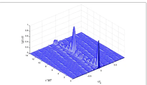
whereu1(t)is a radar pulse waveform. Figure 2 presents a
sample AF of a SF train of unmodulated pulses calculated by using the MATLAB tool.
It is obvious to see that the range resolution of the sig-nal is improved, but there are still prominent sidelobes in delay and ambiguity in Doppler. As a result, LFMs and SF can be combined to mitigate the raging lobes, i.e., SF train of LFM pulses could be used. An example of SF train of LFM is shown in Figure 3.
We compare the AF of a SF train of LFM pulses, as shown in Figure 3, with the AF of a SF train of unmod-ulated pulses as seen in Figure 2. Clearly, by adding the LFM, the range and the Doppler resolutions are improved by canceling the sidelobes along the delay and Doppler axes. As a result, we choose to use the SF train of LFM pulses as the transmit waveforms in our model to obtain both the range and Doppler resolution gain.
4 Target RCS value estimation
In this section, we use the maximum-likelihood (ML) esti-mation algorithm to perform target radar cross section (RCS) parameter estimation [23] in the proposed RSN model. For the ‘Swerling 2’ model, the RCS voltage|λ(u)|
follows a Rayleigh distribution and the I and Q subchan-nels ofλ(u) follow zero-mean complex Gaussian distri-bution with a varianceγ2(the RCS average power value)
λ(u)=λI(u)+jλQ(u) (15)
In addition,n(u) = nI(u)+jnQ(u)follows a zero-mean
complex Gaussian distribution with a varianceσ2for each I and Q subchannel. We express Equation (12) as following
−0.5
0
0.5
0 2 4 6 8 10 12 14
0 0.2 0.4 0.6 0.8 1
τ/tb
ν*MT
|
χ
(
τ
,
ν
)|
Figure 2Ambiguity function of SF train of unmodulated pulses.
−0.5
0
0.5
0 2 4 6 8 10 12 14
0 0.2 0.4 0.6 0.8 1
τ/t
b
ν*MT
|
χ
(
τ
,
ν
)|
Assuming thatynare independent of each other, then the
Therefore, we represent the ML algorithm to estimate the RCS average valueθas
It is equivalent to maximize logf(y)(natural logarithm),
logf(y)=
necessary condition for the ML estimation is
∂
Equation (24) has the unique solution
this solution gives the unique maximum of logf(y). The expectation ofθML(y)is then
nare independent of each
other, it is
As a result, it is an unbiased estimator.
Fisher’s information [24] in this case can be obtained as
Iθ = −Eθ
Taking Equation (28) into account, we can obtain the Cramer-Rao lower bound (CRLB) [24]
Varθ[θ (y)]≥
1 Iθ =
(E2θ+σ2)2
E4N (31)
From (31), we observe that CRLB is inversely propor-tional to the number of radarsNin the RSN, which means that the RSN with large N will have a low CRLB. We draw this conclusion by assuming that the radar pulses are independent (in time and space) and follow a Rayleigh distribution, according to the ‘Swerling 2’ model.
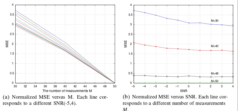
5 Simulation results 5.1 Signal recovery
60 65 70 75 80 85 90 95 100 0
0.5 1 1.5 2 2.5
The number of measurements M
MSE
(a)
Normalized MSE versus M. Each line corre-sponds to a different SNR(-5,4).−5 −4 −3 −2 −1 0 1 2 3 4
0 0.5 1 1.5 2 2.5
M=60
M=95
M=99
M=100
SNR
MSE
(b)
Normalized MSE versus SNR. Each line corre-sponds to a different number of measurements MFigure 4Normalized MSE between reconstructed signal and original signal for fixedN=100.(a) Normalized MSE versusM. Each line corresponds to a different SNR(−5, 4). (b) Normalized MSE versus SNR. Each line corresponds to a different number of measurementsM.
measurementsMand SNR values. The noise considered here is introduced by the propagation in the air but not by compressing and decompressing process. We use the Monte-Carlo simulation model here and the results are averaged by 105runs/iterations. The cases ofN=50 and N = 100, whereNis the number of transmit sensors are illustrated in Figures 4 and 5, separately.
According to both Figures 4a and 5a, MSE is reduced as the number of measurementsMis increased. The sys-tem can perfectly reconstruct the signal which includes
the received signal and the system noise when the num-ber of measurementsMis equal to the number of transmit sensorsN. In addition, the slope of MSE versus the num-ber of measurements Mis almost a consistent for each SNR value. From Figures 4b and 5b, we draw the same conclusion that the closer the number of measurements approachesN(M≤N), the better performance of signal recovery is achieved. In addition, we also discover that the MSE does not depend much on the SNR, especially when Mis large. As a result, the proposed model can be used
30 32 34 36 38 40 42 44 46 48 50
0 0.5 1 1.5 2 2.5 3 3.5 4
The number of measurements M
MSE
(a)
Normalized MSE versus M. Each line
cor-responds to a different SNR(-5,4).
−5 −4 −3 −2 −1 0 1 2 3 4
0 0.5 1 1.5 2 2.5 3 3.5 4
M=30
M=40
M=48
M=50
SNR
MSE
(b)
Normalized MSE versus SNR. Each line
cor-responds to a different number of measurements
M
.
under a low SNR if the number of measurementsMcould be properly chosen according to the number of transmit sensorsN.
On the basis of the simulation results, we can draw a brief conclusion that the number of measurementsMof our model only depends on the size of RSN even when the number of samples is fixed as large as 500 here. Another important result emerging from the simulations is that the probability of target miss detection is zero no matter how small a number of measurements we use in the recovery process. That is to say, less measurements can be used to detect the target in the system, since a kind of diversity gain is achieved at the output of the matched filters on the receiving sensors.
5.2 RCS parameter estimation
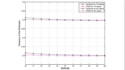
In this section, we will consider the fluctuating target with an RCS parameterθ(following Rayleigh distribution) investigated in the Section 4. We will apply the ML estima-tion algorithm to estimate the parameterθ. The scenario is similar to the one in the section above, but the number of samples in time domain is reduced to 100 for com-plexity reasons. We ran Monte Carlo simulations for 105 iterations at each SNR value. We have considered the fluc-tuating target with RCS parameterθ = 2 (Small flighter aircraft or 4 passenger jet) in Figure 6. We plotted the vari-ance of the RCS ML estimator with different number of radars in RSN.
According to Figure 6, the variance of θ closely approaches the CRLB but doesn’t exactly match it. The reason why the variance ofθis not exactly the same as the CRLB is that the noise included in Equation (10) cannot be termed as sparse as the transmit signal in the same sparsity matrix. Therefore, the noise which is considered in CRLB can not be perfectly reconstructed after the decompres-sion. The power of noiseσ2reduces so that the calculated CRLB might be lower than the practical one. As a result, a gap between the variance ofθ and the CRLB. However, the gap between variance ofθand the CRLB is reduced by increasing the number of radars. It is also easy to see that the actual variance ofθ reduces as the number of radars increases fromN=10 toN =20. Hence, the actual vari-ance ofθis inversely proportional toN, as we have shown in the theoretical result Varθ[θ (y)]≥ (E
2θ+σ2)2 E4N .
It is easy to see that the actual variance ofθ and the CRLB do not change much as the SNR increases. Stat-ing differently, our ML estimator performs well even for low SNR ratios. In all, the simulation results validate the theoretical results. The variance of the RCS parameter estimation satisfies the CRLB and our ML estimator on the RCS parameter is an accurate estimator.
6 Conclusions
Motivated by the representation of SF waveforms, we introduced CS to the RSN exploiting the pulse
10 11 12 13 14 15 16 17 18 19 20 0.2
0.25 0.3 0.35 0.4 0.45 0.5
SNR/dB
Variance of the Estimator
Variance for 10 radars CRLB for 10 radars Variance for 20 radars CRLB for 20 radars
compression technique. A set of SF waveforms were applied as pulse compression codes at the transmit sen-sors, and the sparse matrix is also constructed based on the same SF waveforms. We observed that the sig-nal samples along the time domain can be significantly compressed and recovered by using a small number of measurements which depend on the number of trans-mit sensors. A diversity gain is also achieved after the matched filters in the proposed model, so the probabil-ity of target miss detection can be zero even if the signal could not be perfectly recovered. In addition, we propose a ML algorithm to estimate the target RCS parameter and use the CRLB to successfully verify our theoretical result.
Competing interests
The authors declare that they have no competing interests.
Acknowledgements
This study was supported in part by National Science Foundation under Grants CNS-0964713, CNS-1017662, CNS-0963957, CNS-0964060, and Office of Naval Research under Grant N00014-11-1-0071.
Author details
1Department of Electrical Engineering, University of Texas at Arlington,
Arlington, TX 76010, USA.2Department of Computer Science, The George
Washington University, Washington DC 20052, USA.3Department of
Preventive Medicine and Biometrics Uniformed Services, University of the Health Sciences Bethesda, Maryland 20814-4799, USA.
Received: 25 October 2012 Accepted: 5 January 2013 Published: 19 February 2013
References
1. S Mukhopadhyay, C Schurgers, D Panigrahi, S Dey, Model-based techniques for data reliability in wireless sensor networks. IEEE Trans. Mob. Comput.8(4), 528–543 (2008)
2. T Onel, C Ersoy, H Delic, Information content-based sensor selection and transmission power adjustment for collaborative target tracking. IEEE Trans. Mob. Comput.8(4), 1103–1116 (2009)
3. J Liang, Q Liang, Design and analysis of distributed radar sensor networks. IEEE Trans. Parallel Distrib. Process.22(11), 1926–1933 (2011)
4. H Deng, Synthesis of binary sequences with good correlation and cross-correlation properties by simulated annealing. IEEE Trans. Aerosp. Electron. Systs.8(8), 684–689 (2009)
5. Q Liang, Waveform design and diversity in radar sensor networks: theoretical analysis and application to automatic target recognition. IEEE Sensor Ad Hoc Commun. Netws. Conf.2(28), 684–689 (2006)
6. Q Liang, Radar sensor networks for automatic target recognition with Delay-Doppler uncertainty. IEEE Military Commun. Conf.
23–25, 1–7 (2006)
7. MA Richards,Fundamentals of Radar Signal Processing(McGraw-Hill, 2005) 8. E Candes, M Walkin, An introduction to compressive sampling. IEEE Signal
Process. Mag.25(2), 21–30 (2008)
9. R Baraniuk, Compressive sensing. IEEE Signal Process. Mag.24(4), 118–121 (2007)
10. E Candes, J Romberg, T Tao, Robust uncertainty principles: exact signal reconstruction from highly incomplete frequency information. IEEE Trans. Inf. Theory.52(2), 489–509 (2006)
11. D Donoho, Compressed sensing. IEEE Trans. Inf. Theory. 52, 1289–1306 (2006)
12. E Candes, T Tao, Near-optimal signal recovery from random projections: universal encoding strategies. IEEE Trans. Inf. Theory.52(12),
5406–5425 (2006)
13. R Baraniuk, P Steeghs, inRadar Conf., 2007 IEEE. Compressive radar imaging, (2007), pp. 128–133
14. AC Gurbuz, JH McClellan, WR Scott, inProc. 41th Asilomar Conf. Signals, Syst. Comput. Compressive sensing for GPR imaging, Pacofoc Grove, CA, 2007), pp. 2223–2227
15. AC Gurbuz, JH McClellan, WR Scott, A compressive sensing data acqisition and imaging method for stepped frequency GPRs. IEEE Trans. Signal Process.57, 2640–2650 (2009)
16. S Shah, Y Yu, A Petropulu, in2010 IEEE International Conference on Acoustics Speech and Signal Processing (ICASSP). Step-frequency radar with compressive sampling (SFR-CS), (2010), pp. 1686–1689
17. Y Yu, AP Petropulu, HV Poor, MIMO radar using compressive sampling. IEEE J. Sel. Top. Signal Process.4(1), 146–163 (2010)
18. Y Yu, AP Petropulu, HV Poor, in2010 4th International Symposium on Communications, Control and Signal Processing (ISCCSP). Range estimation for MIMO step-frequency radar with compressive sensing, (2010) 19. S Gogineni, A Nehorai, in2010 International Waveform Diversity and Design
Conference (WDD). Adaptive design for distributed MIMO radar using sparse modeling, (2010)
20. MA Herman, T Strohmer, High-resolution radar via compressed sensing. IEEE Trans. Signal Process.57(6), 2275–2284 (2009)
21. P Swerling, Probability of detection for fluctuating targets. IRE Trans. Inf. Theory.6, 269–308 (1960)
22. N Levanon, E Mozeson,Radar Signals(Wiley, New York, 2004) 23. Q Liang, X Cheng, KUPS: knowledge-based ubiquitous and persistent
sensor networks for threat assessment. IEEE Trans. Aerosp. Electron. Syst. 44(3), 1060–1069 (2008)
24. JM Mendel,Lessons in Estimation Theory for Signal Processing,
Communications, and Control(Prentice-Hall, Upper Saddle River, NJ, 1995)
doi:10.1186/1687-1499-2013-36
Cite this article as:Xuet al.:Compressive sensing in distributed radar sensor networks using pulse compression waveforms.EURASIP Journal on Wireless Communications and Networking20132013:36.
Submit your manuscript to a
journal and benefi t from:
7Convenient online submission 7Rigorous peer review
7Immediate publication on acceptance 7Open access: articles freely available online 7High visibility within the fi eld
7Retaining the copyright to your article