Image-Based Multiresolution Implicit Object Modeling
Augusto Sarti
Dipartimento di Elettronica e Informazione, Politecnico di Milano, Piazza L. Da Vinci 32, 20133 Milano, Italy Email: [email protected]
Stefano Tubaro
Dipartimento di Elettronica e Informazione, Politecnico di Milano, Piazza L. Da Vinci 32, 20133 Milano, Italy Email: [email protected]
Received 5 October 2001 and in revised form 14 May 2002
We discuss two image-based 3D modeling methods based on a multiresolution evolution of a volumetric function’s level set. In the former method, the role of the level set implosion is to fuse (“sew” and “stitch”) together several partial reconstructions (depth maps) into a closed model. In the later, the level set’s implosion is steered directly by the texture mismatch between views. Both solutions share the characteristic of operating in an adaptive multiresolution fashion, in order to boost up computational efficiency and robustness.
Keywords and phrases:object modeling, 3D reconstruction, level-set, surface reconstruction, multi-base-line stereo.
1. INTRODUCTION
Building a complete 3D model of objects from a sequence of images is a task of great difficulty, as it involves many complex steps such as camera motion tracking, image-based depth estimation, and global surface modeling. In order to solve the first problem, a variety of solutions are available ei-ther in the literature or commercially. Aside from the many motion feedback systems available in commerce, the litera-ture is rich with image-based systems that enable a fairly reli-able estimation of the camera motion through the analysis of the acquired video sequences. Such solutions usually exploit projective constraints and invariants to perform image cali-bration [1] and vary in how such constraints are used, how the outliers are managed, and whether additional informa-tion (feature coplanarity, collinearity, etc.) can be included. Alternative camera motion estimation techniques are based on Extended Kalman Filtering and are also available com-mercially and in the literature [2, 3] in more or less sophis-ticated versions. In this paper, we will not be concerned with the problem of camera motion estimation, instead, we will focus on the problem of global surface modeling based on images.
With “global surface” we mean the external (visible) frontier of a volume, which is bound to be a closed surface. Modeling closed surfaces, indeed, poses a number of repre-sentation problems which are typical of differential topol-ogy. Such surfaces, in fact, can be thought of as differentiable
manifolds, and their modeling solutions are closely related to their classical representations.
A 3D manifold can be generally defined and represented eitherexplicitly, through a juxtaposition of overlapping 3D maps; or implicitly, as the set of points that satisfy a non-linear constraint in the 3D space (a level set of a volumetric function). Using the former or the latter, surface represen-tation has a substantial impact on how the image-based 3D modeling problem is posed. An explicit global object model is, in fact, obtained as a “patchworking” of local reconstruc-tions (range images or depth maps), while an implicit sur-face is described as a level set of an appropriate volumetric function. An explicit modeling method deals with topologi-cal complexity with a “divide-and-conquer” strategy, which simplifies the local shape estimation process. The price to pay for this simplification, however, is in the complexity of the steps that are necessary for fusing the local reconstruc-tion into a global closed one (registrareconstruc-tion, fusion and hole-mending). An implicit approach to surface modeling, on the other hand, tends to be more robust against topological com-plexity, as it may easily accommodate self-occluding surfaces, concavities, arbitrary topological varieties (e.g., doughnut-shaped surfaces, objects with handles, etc.), or even multiple objects. On the other hand, an implicit method is bound to work with volumetric data, with more storage requirements and a heavier computational load.
inter-faces in a variety of fields, ranging from computational ge-ometry to materials science [5]. The approach has been stud-ied in depth over the past two decades and a variety of so-lutions have been proposed to overcome some of the basic limitations of the method and to make it as computation-ally efficient as possible. More recently, the level set approach proved effective for several image processing and computer vision applications [6, 7, 8, 9, 10, 11, 12, 13], including image-based 3D surface modeling [14]. In particular, some effective strategies have been proposed to overcome the in-evitable computational costs associated to the intrinsic volu-metric representation in image-based shape modeling. Such solutions refer to two different approaches to image-based surface modeling: the first (indirect method) consists of constructing the global surface as 3D mosaic of simpler sur-face patches [15], while the second (direct method) skips the partial modeling step and uses the available images to steer the evolution of the level set toward the final surface shape [16]. Both methods use a narrow-band approach in conjunc-tion with a multiresoluconjunc-tion technique (adaptive cell size) to boost the performance of surface fusion and image-based 3D modeling techniques. In this paper, we will explore these two methods in depth, discussing the fundamental differences in their implementation strategies and illustrating some imple-mentational aspects of the solutions.
In Section 2, we review some well established basic ideas behind implicit object modeling in the context of image-based surface modeling applications. The purpose of this sec-tion is to provide the readers who are not familiar with im-plicit methods with some helpful ideas to better understand the rest of this contribution . In Section 2, we also antici-pate some technical solutions that we adopted in the spe-cific applications described in the following two sections. In Section 3, we propose a novel application of the ideas set forth in Section 2 to the surface fusion problem. In partic-ular, we discuss how to specialize the front evolution for this particular application and how to obtain optimal per-formance from this approach, both in terms of quality of the results and in needed computational power. Section 4 ad-dresses in depth a second image-based modeling application where front evolution is directly driven by images. Although the approach used for this second application is not new [14], the solutions adopted to boost the performance and cut the computational cost of this implementation are new. This method, in fact, allows to operate in a multiresolution fash-ion. In particular, a careful management of front evolution is proposed, which is able to back-track and recover details lost at lower levels of grid density. Applications to real data are presented in each section, which prove the effectiveness of the approach. Final comments and proposals of improve-ments conclude this contribution in Section 5.
2. IMPLICIT SURFACE MODELING
As already discussed in Section 1, although there are a variety of reasons why an implicit surface representation would be preferable over an explicit one, the most compelling reasons remain the ability to deal with complex surface topologies
and the optimal and simultaneous management of the avail-able image information. In this section we provide the reader with some fundamentals on level set evolution in the context of image-based modelling applications.
2.1. Interface propagation
Our approach to surface modelling is not through piecewise construction, but through interface propagation, that is, the temporal evolution of a closed oriented surface or, more gen-erally, of some oriented surface that separates two regions from each other. This surface will “sweep” the volume of in-terest until it takes on the desired shape under the influence of some properly defined action.
Since we are not interested in any interface motion in its own tangential directions, we can assume this surface to move in a direction normal to itself (either outward or in-ward) with a known velocity functionF. It is in this speed function that we will embed the external action terms, plus the necessary smoothing terms that guarantee a successful convergence of the front to the desired solution. The veloc-ity function, in general, depends on a variety of information sources, which are more or less related to the shape of the front [5], as follows.
Local (intrinsic) properties of the front:local geometric in-formation on the front, such as curvature and normal direc-tion.
Global properties of the front:global information that de-pends on the available data, and that usually dede-pends on the shape and the position of the front (through integration over the front).
Independent properties:external action terms that are in-dependent of the shape of the front.
A proper choice for the velocity function is crucial for the success of the modeling technique. Later in this section we will illustrate some examples of properties that we used for our applications to 3D surface modeling.
There are two distinct formulations of the differential equations that describe interface motion. The first is referred to as boundary value approach, and the second is the initial value approach. Such formulations lead to the fast marching method and the level set method, respectively.
2.1.1 Boundary value approach
If we can assume that the velocity termFis always positive, the characterization of the position of the frontΓ(t) can be entirely given in terms of the arrival timeT(x) of the front as it crosses each pointx=[x1 x2 x3]T,
Γ(t)=x|T(x)=t. (1) The gradient∇Tof this function is bound to be orthogonal to its level sets, therefore it is parallel to the velocity function
F. If we also consider the usual idea that velocity is the ratio between displacement and time, then the arrival functionT
will satisfy the equation
where we haveT=0 on the initial locationΓ(0) of the inter-face. We thus have a formulation of the problem in terms of a PDE (partial differential equations) subject to a boundary condition [5].
2.1.2 Initial value approach
If we want to remove the constraint of monotonic propa-gation and allow the front to move forward and backward, then the crossing time T can no longer be a single-valued function. We thus need to adopt an alternative representa-tion for the front. An appropriate choice is to represent the initial front as the zero level set of a volumetric functionφ. We can then link the evolution of this function to the prop-agation of the front through a time-dependent initial value problem [8, 9, 10, 17]. The front, in fact, will be given by
Γ(t)=x|φ(x, t)=0. (3) The equation of the motion can be easily derived by im-posing that a particle on the front with trajectoryx(t) lies on the zero level set of the volumetric function
φx(t), t=0, (4)
and that the normal component of its velocity matchesF
∂x(t)
∂t ·n=F, (5)
wheren= ∇φ/|∇φ|.
Differentiating the left-hand side of (4)
∂φ ∂t +
∂x(t)
∂t · ∇φ= ∂φ
∂t + ∂x(t)
∂t ·n|∇φ|, (6)
and using (5), the initial value problem [17] can be rewritten as
∂φ
∂t +F|∇φ| =0, (7)
givenφ(x,0). Equation (7) can be discretized into the update equation
φ(x, t+∆t)=φ(x, t)−∇φ(x, t)F(x)∆t. (8) It is important to emphasize the fact that now there is no a priori condition on F, which can be arbitrary. In partic-ular, its sign is free to change, therefore the front can move forward and backward as it evolves. This particular PDE be-comes a special case of the Hamilton-Jacobi equation if the speed depends only on positionxand first derivatives ofφ.
In applications of computer vision and 3D modeling, the structure of the embedding volumetric functionφis not nat-urally suggested by the nature of the problem, therefore we can invoke the need to keep computations as simple as possi-ble and decide on a volumetric function whose absolute value inxis given, the distancedbetweenxand the evolving front and its sign depends on whether the pointxis inside or out-side the surface. Adopting the signed distance as a volumetric
function, in fact, simplifies the computation of the surface’s differential properties [5] of orders 1 and 2:
(i) the surface normal can be computed as the gradient ∇φand is a unit vector;
(ii) the surface curvature can be computed as a divergence of the form∇ · ∇φ.
2.1.3 A comparison
It is important to notice that (2) requiresF >0 all the time, which means that the front is expected to move always in the same direction, because it must generate one single crossing time per grid point (points cannot be revisited). This is, in-deed, a very strong requirement that should be avoided in image-driven surface shaping schemes, especially if working in with variable grid resolution. In fact, if we happen to miss some surface details at a certain grid resolution, we need to be able to backtrack the evolution and retrieve the lost details as we increase its resolution.
Also, the framework of initial value level set methods allows to define the speed function in a quite arbitrarily complex fashion. This gained freedom, however, has a price in terms of computational efficiency. Fast marching meth-ods, which are efficient implementations of boundary value methods, benefit from the fact that the time of arrival is a single-valued map to compute the front evolution in a single sweep, using heap-sort algorithms to generate the grid’s vis-iting order. In spite of the loss of efficiency, level set methods, which are direct implementations of initial value solutions, can be made quite efficient through a joint use of narrow band and adaptive mesh strategies [5]. Because of these rea-sons, and others that will be illustrated throughout the paper, we adopt a level set approach for our surface modeling solu-tions.
2.2. Front stability and smoothness
Figure1: Motion by curvature: the surface deflates in a maximally smooth fashion until it disappears.
The necessity of a smoothing term is also justified by the need of overcoming the intrinsic ill-conditioning of stereo problems and, more generally, of computer vision problems.
2.3. Narrow band
Updating the volumetric function whose level set zero rep-resents the propagating front requires, in principle, the up-dating ofO(M3) voxels,Mbeing the linear size of the voxset (expressed in voxels). A Lagrangian (particle tracking) ap-proach, on the other hand, is only expected to update the location of the points of the propagating front, therefore we only need to act onO(M2) points. This excess in the compu-tational cost associated to a level set approach is due to the intrinsic redundancy of an implicit surface representation, but it can be drastically reduced if we consider that the vol-umetric functionφdoes not need to be updated everywhere, as we are only interested in the zero level set of φ. In fact, only the values ofφin the proximity of the front tend to have an influence on the evolution of its shape, due to the spa-tial derivatives that appear in the PDE that governs the front propagation. As a consequence, it is possible to limit the re-gion of influence to a “narrow band” (NB) centered around the evolving front
x∈NB⇐⇒φ(x)≤δ
2, (9)
δbeing the thickness of the narrow band [12, 18]. As a conse-quence, the number of voxels to be updated is back toO(M2). We have to keep in mind, however, that the inevitable dis-cretization errors that occur in the implementation of the equation that governs the front evolution require an occa-sional reinitialization of the volumetric function within the narrow band, with the constraint of keeping the front un-changed. The choice of the thicknessδ must be a trade-off
between the need of minimizing the number of voxels to up-date and minimizing the number of reinitializations. Typi-cally,δis set to values that range between 10 and 20 voxels.
A straightforward way to implement the updating pro-cess for NB reinitialization is based on the recomputation of the distance function from the front. This operation, how-ever, is computationally expensive, therefore we adopt an it-erative approach to do so. The method consists of a first rough reinitialization of the volumetric function, followed by an iterative refinement process that returns the actual signed distance function from the front. This iterative process is meant to change the function in order for its gradient to have a unit magnitude. This is, in fact, done by discretizing a spe-cial type of Hamilton-Jacobi PDE [19],
∂φ ∂t =sign
φ0
·1− |∇φ|, (10)
whose solution is a distance function φ (|∇φ| = 1) and whose level zero is the initial function φ0. This iterative scheme turns out to be far more efficient than a complete reinitialization, especially if the rough initializationφ0is al-ready quite accurate [20]. One way to build a good approx-imationφ0of the desired functionφis to keep the previous values. Of course, as the front migrates between two reini-tializations, we will be able to use only some of the previous values. The other voxels (those that are located in the new portions of the narrow band) will be assigned increasing (de-creasing) values as we move outward (inward) with respect to the front.
This method [21] has been proven to be equivalent to the so called “upwind scheme” [5], which is based on an appro-priate choice of the discretization of the partial diff erentia-tion operator.
2.4. Multiresolution
As already said above, working in a narrow band around the propagating front dramatically reduces the number of voxels to be updated fromO(M3) toO(M2). A further drastic re-duction in the updating complexity comes from the adoption of a multiresolution strategy in the front evolution, which drops the complexity to a mereO(MlogM). The term mul-tiresolution, however, requires some explanation, as it may lead to completely different solutions in the data structure and management. In particular, if we do not know in advance where the surface details are located (direct, or image-driven, shape modeling), all we can do is to let the front evolve on a coarse grid, and increase the voxset resolution of a factor two (23 =8 smaller voxels for each coarser one) every time the front evolution comes to a stop (equilibrium configuration). When the location of the surface details is known (indirect, or surface-driven, modeling), we can do better than just per-form an on-the-fly split of the whole voxset. In fact, we can reorganize the data structure in a hierarchical fashion using an octree. This, of course, complicates the computation and the management of the derivatives and of the velocity func-tion, but it boosts the performance even further.
applications (indirect and direct modeling) proposed in the next two sections.
2.5. Construction of the extension velocities
It is important to point out that the velocity function is usu-ally defined only on the propagating frontΓ(t) (zero level set of φ). On the other hand, in order to be able to integrate the PDE that governs the motion of the propagating front, we need the speed function to be defined on the whole do-main of interest of φ, which is the narrow band defined in Section 2.3. The extension of the velocity function in that do-main must be done starting from its profile on the propagat-ing front, in such a way to guarantee that the evolution ofφ
in the whole narrow band will be consistent with evolution of the propagating front [22]. Roughly speaking, we would like all level sets ofφto propagate without self-collisions (swal-lowtail configurations) or rarefactions (gaps).
In order to define an extension of the velocity function that does not generate self-collisions or rarefactions, we can proceed as follows: letΓ= {x|φ(x)=0}be the propagating front and consider a generic pointxP. IfxPdoes not lie on
Γ, we can always find another level set that it belongs to. In other words, we can always find acsuch thatφ(xP)=c. If
xQ=arg min
xQ∈Γ
xQ−xP (11)
is the closest point ofΓtoxP, then we can assignxPthe ve-locity F(xP) = F(xQ). This operation can be done for ev-ery point of the narrow band, and is exempt from the above-mentioned problems of self-collision or rarefaction [5].
2.6. Volumetric and surface rendering
Visualizing the zero level set of a volumetric function is im-portant when we need to visually follow the evolution of the front. Conventional surface visualization techniques, how-ever, are suitable for Lagrangian surface descriptions (trian-gle mesh), but they do not directly apply to an implicit sur-face representation. In this section, we discuss a solution for visualizing the evolving front, without having to construct the surface mesh.
The method consists of assigning a luminance value to a generic pixel through the analysis of sign changes in the volumetric functionφalong the associated optical ray:
(i) if the volumetric functionφ(x) does not change sign along the optical ray, we assign the pixel the back-ground luminance;
(ii) ifφ(x) exhibits a sign change along the optical ray, then the pixel will be assigned a value of luminance, com-puted using an appropriate radiometric model that ac-counts for the viewing direction and the normal to the front. In fact, we assume the local texture to be lo-cally uniform and the light to be diffused, the lumi-nance will only depend on the viewing direction (non-Lambertian component)
I= i·n
in, (12)
whereiis the viewing direction andnis the front’s nor-mal in the considered point, which can be computed directly from the samples ofφthat surround the point along the optical ray, whereφchanges sign.
It is also quite easy to map other characteristics on the evolving front, such as the cost function or the original tex-tures. As for the final model, the conversion to a more con-ventional wireframe can be easily performed using a modi-fiedmarching cubesalgorithm [23].
3. INDIRECT SURFACE MODELING
A common way to build a complete 3D object model consists of combining several simpler surface portions [24, 25, 26] (range images or depth maps) through a 3D “mosaicing” process. In order to do so, we need a preliminary registra-tion phase [27], in which all the available surface patches are correctly positioned and oriented with respect to a com-mon reference frame; and a fusion process, which consists of merging all surface patches together into one or more closed surfaces. One rather standard registration strategy is the It-erative Closest Point [28] algorithm, which consists of min-imizing the mean square distance between overlapping por-tions of the surface, using an iterative procedure. As for sur-face fusion, in this section we propose and test an approach that is able to seamlessly “sew” the surface overlaps together, and reasonably “mend” all the holes that remain after sur-face assembly (usually corresponding to non-visible sursur-face portions).
This patchworking process is suitable for combining 2D 1/2 modeling solutions such as image-based depth estima-tion techniques, range cameras, and laser scanners. It is im-portant to stress that the depth maps produced by such devices could be made of several non-connected surface patches, as occlusions and self-occlusions tend to gener-ate depth discontinuities [26]. Such surfaces usually need a lengthy assembly process in order to become a complete and closed surface.
3.1. Definition of the velocity function
The velocity function that steers the front evolution accounts for two contrasting needs: that of generating a smooth front propagation with no degenerate configurations (motion by curvature) and that of honoring the data (oriented surface patches). As already seen in the previous section, if the mo-tion were purely by curvature, a surface would tend to de-flate completely and disappear, while becoming progressively smoother and smoother (Figure 1). The need to honor the available range data prevents this complete implosion from taking place.
produce unpleasant front profiles in the proximity of discon-tinuities between different surface portions. A better front behavior is obtained by replacing the product with a simple sum of the two above terms. This solution, however, tends to round all edges, with a consequent loss of accuracy. In or-der to avoid this problem, we define the velocity function as
F(x)=F1
k(x)+αkM(x) k(x) F2
d(x), (13)
wherekis the front’s local curvature,kM is the local curva-ture of the facing surface;dis the distance (with sign) be-tween the propagating front and the surface patch; andαis a weight that balances the two terms of local smoothness and data fitting. In this version of the velocity function, the term that promotes data fitting is multiplied by a corrective factor that depends on the local curvature of the surfaces that are facing the front. This tends to encourage the front to fit the data much more in the proximity of edges.
Notice that the above definition of velocity is only valid on the propagating front, therefore we need to extend it to the whole volume of interest (narrow band around the prop-agating front), as explained in Section 2.3.
3.2. Precomputation of the distance function
One crucial step of the indirect method is the computation of the distance function that appears in (13), which charac-terizes the data-fitting term of the velocity function. The zero level set of this function gives a rough idea of the global shape and of the level of detail that the final model will have, there-fore it allows to correctly decide initial and final spatial dis-cretization steps. In fact, the initial voxset resolution must be sufficient to capture the topology of the surface to model, while the final voxset resolution must be adequate to model the surface details.
It is important to emphasize that the distance function can be computed on the whole volume of interest before starting the front evolution. Given a generic pointx, its dis-tance from a single oriented surface can be easily computed as the distance betweenx and its projection onto the clos-est triangle of the mesh (Figure 2). If no point on the surface patch faces the point on the level set orthogonally, then the distance functiondis computed from the closest point on the border of the patch (within certain angular limits). Of course this distance will be attributed a sign, depending on which side of the surface the pointxis facing. In particular, negative values of the distance function tend to prevent the front from penetrating apertures or holes between surface portions and avoids useless concavities. Indeed, this computation leads to a distance whose zero level set coincides with the initial sur-face.
In the presence of several surfaces, the distance must be computed as a combination of the various distances (within reasonable limits), taking into account, somehow, their reli-ability. Indeed, a special case is represented by two overlap-ping surfaces that are oppositely faced, and need to be treated separately (in this case the viewpoints are in opposition).
x1
n1 P1
x2
n2
P2
Figure2: Distance function in the case of a single surface.
Also, we need to exclude all surface portions that, although correctly oriented, are too far apart from the considered point.
If we consider thekth mesh of triangles,k=1, . . . , N, we can compute the distancedk(x) from the pointxas follows:
(1) find the closest nodemtox;
(2) find the pointpthat lies the closest tox, on the trian-gles that share the node as a vertex;
(3) computedk(x) as follows:
(i) ifpis not a frontier point of the triangle mesh, then
dk(x)=(x−p)·n;
(ii) ifpis a frontier point of the triangle mesh, then
dk(x)=
+(x−p) when (x−p)·n ≥0,
−(x−p) when (x−p)·n<0. (14)
The zero level set ofdk(x) turns out to be continuous and piecewise linear, just like the original triangle mesh.
In order to compute the global distance function d(x) that pertains a set of multiple surfaces, we can proceed as follows:
(1) find the algebraic distancedk(x),k = 1, . . . , N, from each available mesh;
(2) if all distances correspond to border points, then let
d(x)=dmin(x), (15)
otherwise go to step 3.
(3) letdmin(x) be the smallest of all distances dk(x) that are not measured from a border point. Let pmin be the point from which that minimum distance is com-puted,nminbe the surface normal at that point, and
I=k|nk·nmin
>0 (16)
be the set of indices that identify all surfaces oriented like nmin, nk being the normals at the other closest non-border points. Similarly, we can determine the set of surfaces oriented opposite tonmin
I=k|nk·nmin
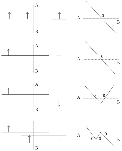
A
B A
B A
B
B
A 0
B
A 0
B
A 0 0
B
A
0 0 0
B
Figure3: Distance function in the case of multiple surfaces. Left: surface sections with the relative normals. Right: distance profile along section A-B.
At this point we can determinedopp(x) as the distance with minimum magnitude among those that are ori-ented opposite tonminand use this value as a thresh-old to rule out ofI all distances whose magnitude is greater thandopp(x). We can thus computed(x) as a linear combination of the remaining points of the setI
d(x)= i∈I
widi(x), (18)
wherewiare properly chosen weights.
In Figure 3, we can see some examples of distance pro-files corresponding to uniform weights wi. As a matter of fact, the choice of the weights wi can be critical for a fine tuning of the result, as they allow to decide whether to trust one surface patch better than another one. Indeed, if we had a priori information on the accuracy and the reliability of a partial reconstruction, it would be easy to use this infor-mation through a careful choice of the weights. In our case, however, this information is not available. However, we can always infer an appropriate weight configuration on a heuris-tic basis. For example, if we are using an image-based depth estimation technique to obtain the partial reconstructions (range images), we can safely assume that the least reliable surface portions are those that lie in the proximity of self-occlusions or extremal boundaries. It is thus reasonable to assign a higher weight to regions that are far from the border. Another reasonable criterion can be used whenever the over-lap involves several surfaces. In this case it is reasonable to limit the averaging only to those surfaces that remain within
5 10 15 20 25 30
5 10 15 20 25 30
10 20 30 40 50 60 10
20 30 40 50 60
20 40 60 80 100 120 20
40 60 80 100 120
Figure4: Multiresolution progression of the voxset where the vol-umetric function is defined.
a certain distance from each other. This tends to rule out pos-sible outliers in the partial reconstructions. One final pospos-sible parameter that could be easily considered in the computa-tion of the distance funccomputa-tion is surface orientacomputa-tion. In fact, if we knew the viewpoint associated to a certain partial recon-struction, we could decide to favor those surface areas that are more orthogonal to the viewing direction.
3.3. Multiresolution
Of course, we also need to recompute the distance function through an iterative process that is similar to the one used for the reinitialization of the narrow band (see Section 2.3).
The initial resolution must be set in such a way to be able to obtain a fast front evolution, without missing surface de-tails. In fact, the voxel size should be decided in such a way to guarantee a correct sampling of all scene elements of interest. Failing to do so would result in a front that “passes through” some surface elements.
A key aspect of this process is the fact that the velocity field that drives the implosion of the level set can be pre-computed on a hierarchical data structure (octree that best fits the available range data).
The resulting model is bound to be a set of closed sur-faces, therefore all the modeling holes left after mosaicing the partial reconstructions are closed in a topologically sound fashion. In fact, those surface portions that cannot be re-constructed because they are not visible, can sometimes be patched up by the fusion process. This ability to mend the holes can also be exploited in order to simplify the 3D acqui-sition session, as it allows to skip the retrieval of some depth maps.
An interesting aspect of our fusion method is in the pos-sibility to modify the surface characteristics through a pro-cessing of the volumetric function. For example, filtering the volumetric function results in a smoother surface model. Fi-nally, the method exhibits a certain robustness against orien-tation errors, as the non perfect matching of surface borders can be taken care of by the fusion process through a careful definition of the distance function used in the specification of the volumetric motion field.
3.4. Examples of application
In order to test the effectiveness of the proposed technique, we applied it to a variety of study cases. A series of tests on synthetic data were conducted to confirm the system’s ability to deal with complex topologies, with multiple objects, with facing surfaces, and with hole-mending situations. In partic-ular, some tests on multiple facing surface were conducted on the synthetic data set (the handle of a pitcher chained to a torus), proving that the definition of the distance function for multiple surfaces, provided in Section 3.2, is effective (see Figure 5).
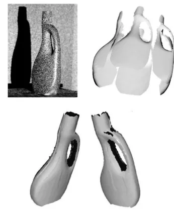
A particularly interesting experiment was conducted on a real object with a nontrivial topology (a bottle with a han-dle) that could easily create problems of ambiguities. Any tra-ditional surface fusion approach would, in fact, encounter difficulties in deciding how to complete (close) the surface in the regions of missing data. Furthermore, besides exhibit-ing self-occlusion problems, this object puts the multireso-lution approach under a severe test. We acquired six depth maps and assembled them together using an ICP algorithm [28] (see Figure 6). The result was an incomplete model with some accuracy problems in the overlapping regions (at the boundaries of the depth maps). The front evolution is shown in Figure 7, which results in the final model of Figure 8.
As we can see, the topology of the object is retrieved cor-rectly, without having to provide the system with specific
Figure5: Testing the distance function: progressive reconstruction of a surface of complex topology with multiple facing surfaces.
Figure6: One of the original views (top left). Six unregistered sur-face patches obtained with stereometric techniques (top right). Two views of the assembled surface patches after registration (bottom): notice the creases due to a nonperfect model overlapping, and the presence of holes in the global model.
instructions. Also, through a simple low-pass filtering of the volumetric function, we can reduce the problems that oth-erwise would arise from the jaggedness of the borders of the surface patches.
4. DIRECT SURFACE MODELING
Figure7: Level set implosion.
Figure8: Final 3D model.
working on a narrow band around the evolving front, it op-erates in an adaptive multiresolution fashion, which boosts up the computational efficiency. Multiresolution, in fact, en-ables to quickly obtain a rough approximation of the objects in the scene at the lowest possible voxset resolution. Succes-sive resolution increments allow to progresSucces-sively refine the model and add details. In order to do so, we introduce sev-eral novel action terms in the velocity function, which al-low to control the front evolution in the desired fashion. For example, we introduce “inertia” in the level set evolution, which tends to favor topological changes (e.g., the creation of doughnut-like holes in the structure). Other mechanisms that implement some sort of biased quantization and hys-teretic evolution tend to prevent its dynamics from missing details (surface creases, ridges, etc.) at lower resolution levels, or to recuperate them at every resolution increment.
4.1. Definition of the velocity function
One of the terms that contribute to steering the level set evo-lution is the texture mismatch between imaged and trans-ferred textures [24, 25], which is a function of the correlation between homologous luminance profiles [29]. The texture
mismatch is the surfaceS, associated to the local surface parametrization (v, w) induced by the image coordinate chart;n is the sur-face normal; andIi(mi) is the luminance of pixelmiin the
ith image. This definition ofdσ guarantees that the surface representation will be independent of the variables (u, w). The surface patchS through which the luminance transfer occurs is assumed to be a locally planar approximation of the propagating front. Indeed, in order to guarantee that this ap-proximation will maintain a constant quality, the size of this planar patch will change according to the local curvature of the level set.
The inner product (correlation) between the pair of subimagesIiandIjis defined as follows:
where m1 andm2 are homologous image points (i.e., im-age points that correspond to the same point of the surface model), and
Although the correlation could be computed between all the viewpoints where there is visibility, only the pair of views with the best visibility is considered. Visibility can be easily checked through a ray-tracing algorithm and measured as a function of the angle between visual ray and surface normal. Notice that normalizing the correlation has a twofold pur-pose: to limit its range between 0 and 2; and to guarantee that low energy areas (smooth texture) will have the same range of high energy (rough texture) areas. Finally, subtracting the average from a luminance profile tends to compensate a non-Lambertian behavior of the imaged surfaces.
In order to achieve the desired front evolution, we pro-pose and define a novel velocity function that mediates the twofold need of guaranteeing surface smoothness and con-sistency between images and final model
F(x)=C(x)divφ+∇ψ· ∇φ+αψ. (23)
Texture-curvature action
Hook-on action
Ideally, we would be lead to think that the first term is suffi-cient to correctly steer the model’s evolution, as correct sur-face regions should have a zero cost, while other regions are left free to evolve. This, however, is not really true as the cost is rarely equal to zero due to a nonperfect luminance trans-ferral (a homography models just a first-order approxima-tion of the surface) and a non-Lambertian radiometric be-havior. Because of that, without some additional contrasting action, the front propagation would “trespass” the correct surface and continue its evolution uncontrollably. The sec-ond term of (23) will tend to contrast this behavior. In fact, in the proximity of the actual surface, the local cost gradi-ent∇ψis almost parallel (although oppositely oriented) to the propagation front’s normaln = ∇φ. As a consequence, ∇ψ· ∇φ <0 tends to stabilize the front in the proximity of the actual surface. Furthermore, this term exhibits the desir-able property of speeding up the evolution of the front in the proximity of configurations of minimum cost, as it accounts of a positive action∇ψ· ∇φ >0.
Inertia action
The third term of (23) acts like an “inertial” term in order to favor concavities in the final model. The weight factorα >0 is constant all over the front, but it is variable in time. In fact,
αmust satisfy two opposite needs: on one hand its magnitude needs to be small enough to avoid affecting the action of the first term of (23); on the other hand, it has to be large enough to produce the desired topological changes. We found exper-imentally that a good choice forαcorresponds to the average curvature of the front at every time step
α=
S|div φ|dσ
Sdσ
. (24)
The weightαneeds to be rather frequently updated, some-times at every iteration. However, this operation does not re-quire additional computational effort, as the first action term of (23) already requires the computation of divφ.
4.2. Multiresolution
If the volumetric function that characterizes the level set is defined on a static voxset ofN×N×Nvoxels, the compu-tational complexity of each front propagation step is propor-tional toN2, as it is proportional to the surface of the level set (narrow-band computation). Furthermore, since the ve-locityFis multiplied by|∇ψ|(which is equal to the sampling step), the number of iterations turns out to be proportional toN, with a resulting algorithmic complexity that is propor-tional toN3. In order to dramatically reduce this complexity, we developed a multiresolution approach to level set evolu-tion. The algorithm starts with a very low resolution level (a voxset of 10–15 voxels per side). When the propagation front converges, the resolution increases and the front resumes its propagation. The process is iterated until we reach the de-sired resolution. A progressive resolution increment has the desired result of minimizing the amount of changes that each
Multiresolution Single resolution
# iterations
Φ
Figure9: Illustration of the temporal evolution of the cost function (texture mismatch) and of the model. Notice that the cost value sud-denly increases at every resolution change, due to the mechanism of recovery of details.
propagation step will introduce in the model, with the result of achieving a better global minimum of the cost function. Furthermore, the number of iterations will be dramatically reduced (fromNto logN) with respect to a fixed-resolution approach, with an algorithmic complexity that turns out to be proportional toN2logN.
Indeed, starting from a low-resolution voxset, we need to prevent the algorithm from losing details at that resolution or to make sure that the algorithm will be able to recover the lost details. In fact, we have to keep in mind that the motion by curvature tends to dominate over the other terms, there-fore some of the details of the object may totally disappear. In order to prevent this from happening, we limit the impact of the local curvature on the front’s evolution through a “soft” clipping function, which guarantees a better evolutional be-havior than hard clipping.
(a)
(b)
(c)
Figure10: Detail recovery in an object with relevant small details of high curvature. Original image (a), evolution with no backtracking (b), backtracking re-expansion (c).
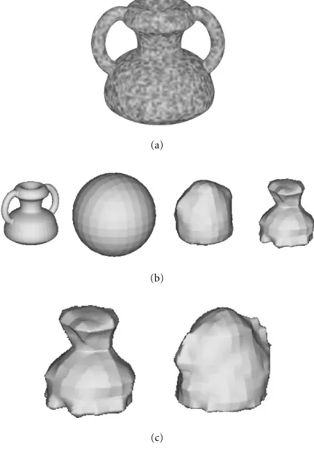
Two are the critical aspects associated to a resolution change: the management of resolution changes; and the re-covery of lost details. The first problem can be approached with a simple interpolation with half the sampling step, fol-lowed by a low-pass filter. The second problem is far more complex, and deserves further discussion.
The basic idea is to select the minimum resolution that allows the front evolution to proceed, without worrying too much about lost details. The final resolution, of course, will depend on the accuracy of the details that we want to repre-sent. Consider, for example, the object of Figure 10a, which exhibits relevant details of small size and high curvature. If we let a low-resolution level set (10×10×10 voxels) evolve under the influence of the above described velocity terms, we obtain the evolution shown in Figure 10b. The algorithm can initially sense the presence of the pitcher’s handles, as the evolving front slows down in their proximity. The front, however, ends up missing the handles completely. This is mainly due to the curvature component of the velocity func-tion, which tends to flatten the front. In fact, any detail whose curvature radius is smaller than the voxel size is filtered out by the front evolution. Roughly speaking, if the resolution is too low, the handles are treated like a ripple to be removed.
−3 −2 −1 0 1 2 3
k 1
0.8 0.6 0.4 0.2
−0.2
−0.4
−0.6
−0.8
−1
Figure 11: Plot of the soft thresholding functionβtanh(k), with β=1 (typical value for most applications).
We recall that the texture-curvature term in the velocity func-tion is the product between texture mismatchψand the cur-vature∇ · ∇φof the front, therefore although the mismatch
ψ becomes very small as the front passes through the han-dles, the curvature factor becomes very large, with the result that the corresponding velocity term does not become zero and the front continues to advance.
In order to avoid this problem, we limit the impact of the front’s local curvature through a “soft clipping” function (see the hyperbolic tangent function of Figure 11). The value ofβ
represents the limit we set for the curvaturek= ∇ · ∇φ, and it is usually set to 1.
Although this soft clipping process is effective in many situations, some complex topologies such as the one of Figure 10a, cannot be correctly reconstructed when starting from a coarse initial resolution. For this reason, we imple-mented a method for recuperating the lost details before a resolution change. The idea is to keep track of the coordi-nates of all the voxels of the zero level set where the texture mismatchψis lower than a certain thresholdε. It is quite rea-sonable to expect that this setᏼof points correspond to all details that have been missed at the previous resolution level. After the front evolution settles to an equilibrium configu-ration, the algorithm begins a backtracking phase in which the front expands toward the points of the setᏼ. In order to do so, we use such points as attractors by adding a new action term in the velocity function, which accounts for the distance from such points.
As we can see in Figure 10c, the point cloudᏼ(here cor-responding to the pitcher’s handle) attracts the closest points of the front in order for the next implosion, which will occur at a higher resolution level, to begin from a model that con-tains all the previously lost details. In Figure 10c we can see the front evolution during the re-expansion phase.
4.3. Implementational issues
Figure12: Sequence of original views.
Figure13: A view of the cost function mapped onto the propaga-tion front. The darker the texture is, the heavier the mismatch.
This operation alone results in a saving of about 50% of the total computational time. Significant computational savings also arise from the choice of computing the luminance agree-ment only on two images at a time (n=2 in (20)) [14].
As for the algorithmic automaticity, we devised and im-plemented a number of solutions that reduce the interven-tion of the operator to a minimum. For example, the algo-rithm selects, for each surface point, the best pair of cameras (C1, C2) for the computation of the correlation (21). This is done by selecting the cameras whose viewing direction is most parallel to the surface normal and whose view of the point is not occluded.
Another important problem to assess is the choice of the width of the window used for computing the correla-tion between textures. In fact, in order to keep computa-tional complexity at a reasonable level, luminance transfer between views is performed through the local tangent plane to the surface (homography). This window cannot be too ex-tended otherwise texture warping would come in the way, but it cannot be too small, otherwise we would have prob-lems of matching ambiguity. What we did in our implemen-tation is to link the window size to the radius of curvature of the evolving front through a simple proportionality relation-ship. In fact, the radius of curvatureρcan be derived imme-diately as the reciprocal of the divergence of the volumetric function.
4.4. Examples of application
In order to prove the effectiveness of our approach to 3D modeling, we tested it on several objects acquired with a camera moving around them. In this section, we show the results in two different cases characterized by a significantly
Figure14: Temporal evolution of the propagation front. The initial volumetric resolution is very modest (in this case the voxset size is 20×20×20), and is not able to account for some topologically complex details of the surface (the fifth frame in lexicographic order is the best one can do at this resolution). As the resolution increases, more details begin to appear, such as the stem of the apple.
Figure15: Four views of the final 3D model.
Figure16: Two of the original views of the subject.
Figure17: Temporal evolution of the propagation front.
performed some experiments in which the images were ac-quired with a modestly cluttered background, without sig-nificantly affecting the evolution of the front.
5. CONCLUSIONS
In this paper we discuss two image-based 3D modeling meth-ods based on a multiresolution evolution of a volumetric function’s level set. The first consists of fusing (“sewing” and “stitching”) numerous partial reconstructions (depth maps) into a closed model, while the second consists of steering the level set’s implosion with texture mismatch between views. Both solutions share the characteristic of operating in an adaptive multiresolution fashion, which boosts up compu-tational efficiency and robustness.
Both modeling applications have been written in C++, and run on several SW platforms. Computational times de-pend on the final resolution and on the topological complex-ity of the imaged object. Using a PC equipped with a Pen-tium III 800 MHz with a 256 MB RAM, the fusion algorithm always completes its task in just a few minutes on voxsets of 128×128×128 voxels. A bit more intensive is the direct ap-proach, mostly because none of the computation can be done in advance. In this case, although the implementation is not optimized, we need less than 10 minutes per resolution level.
Figure18: Final 3D model. The rendered view is here blended with a model’s wireframe, obtained after mesh simplification.
We are currently working on a new version of the above methods, based on 3D mesh adaptivity, which will further improve the computational efficiency and the effectiveness of the solution. We are also working on an image-based au-tomatic fine tuning of the algorithm’s parameters.
REFERENCES
[1] R. Hartley and A. Zisserman,Multiple View Geometry in Com-puter Vision, Cambridge University Press, Cambridge, UK, 2000.
[2] A. Dell’Acqua, A. Sarti, and S. Tubaro, “Effective analysis of image sequences for 3D camera motion estimation,” in
Intl. Conf. on Augmented, Virtual Environments and Three-Dimensional Imaging (ICAV3D 2001), Mykonos, Greece, 30 May–1 June 2001.
[3] A. Azarbayejani and A. Pentland, “Recursive estimation of motion, structure, and focal length,” IEEE Trans. on Pattern Analysis and Machine Intelligence, vol. 17, no. 6, pp. 562–575, 1994.
[4] J. A. Sethian, An analysis of flame propagation, Ph.D. thesis, Department of Mathematics, University of California, Berke-ley, Calif, USA, 1982.
[5] J. A. Sethian, Level Set Methods and Fast Marching Meth-ods, Cambridge University Press, Cambridge, UK, 2nd edi-tion, 1996.
[6] V. Caselles, F. Catte, T. Coll, and F. Dibos, “A geometric model for active contours in image processing,” Numer. Math., vol. 66, no. 1, pp. 1–31, 1993.
[7] R. Malladi and J. A. Sethian, “A unified approach for shape segmentation, representation and recognition,” Tech. Rep. 614, Center for pure and applied mathematics, University of California, Berkeley, Calif, USA, 1994.
[9] R. Malladi and J. A. Sethian, “Level set methods for curva-ture flow, image enhancement, and shape recovery in medi-cal images,” inVisualization and Mathematics, pp. 329–345, Springer-Verlag, Heidelberg, Germany, June 1995.
[10] R. Malladi, J. A. Sethian, and B. C. Vemuri, “Shape modeling with front propagation: A level set approach,”IEEE Trans. on Pattern Analysis and Machine Intelligence, vol. 17, no. 2, pp. 158–175, 1995.
[11] R. Malladi and J. A. Sethian, “A unified approach to noise removal, image enhancement, and shape recovery,” IEEE Trans. Image Processing, vol. 5, no. 11, pp. 1554–1568, 1996. [12] R. Malladi, J. A. Sethian, and B. C. Vemuri, “A fast level set
based algorithm for topology-independent shape modeling,”
J. Math. Imaging Vision, vol. 6, no. 2/3, pp. 269–290, 1996. [13] R. Malladi and J. A. Sethian, “Level set and fast marching
methods in image processing and computer vision,” inProc. IEEE International Conference on Image Processing, Lausanne, Switzerland, September 1996.
[14] R. Keriven, Equations aux D´eriv´ees Partialles, Evolution de Courbes et de Surfaces et Espaces d’Echelle: Applications `a la Vi-sion par Ordinateur, Ph.D. thesis, ´Ecole Nationale des Ponts et Chauss´ees, Paris, France, 1997.
[15] A. Sarti and S. Tubaro, “A multiresolution level-set approach to surface fusion,” inProc. IEEE International Conference on Image Processing, Thessaloniki, Greece, October 2001. [16] A. Colosimo, A. Sarti, and S. Tubaro, “Image-based object
modeling: a multiresolution level-set approach,” inProc. IEEE International Conference on Image Processing, Thessaloniki, Greece, October 2001.
[17] S. Osher and J. A. Sethian, “Fronts propagating with curva-ture dependent speed: Algorithms based on Hamilton-Jacobi formulations,” J. Computational Phys., vol. 79, no. 1, pp. 12– 49, 1988.
[18] R. Malladi and J. A. Sethian, “AnO(NlogN) algorithm for shape modeling,”Proc. Nat. Acad. Sci. U.S.A., vol. 93, no. 18, pp. 9389–9392, 1996.
[19] M. Sussman, P. Smereka, and S. Osher, “A level set approach for computing solutions to incompressible two-phase flow,”J. Computational Phys., vol. 114, pp. 146–159, 1994.
[20] M. Sussman and E. Fatemi, “An efficient, interface preserving level set re-distancing algorithm and its application to inter-facial incompressible fluid flow,” SIAM Journal on Scientific Computing, vol. 20, no. 4, pp. 1165–1191, 1999.
[21] R. Keck, Reinitialization for Level Set Methods, Dipl. the-sis, University of Kaiserslautern, Department of Mathematics, Kaiserslautern, Germany, June 1998.
[22] D. Adalsteinsson and J. A. Sethian, “The fast construction of extension velocities in level set methods,” J. Computational Phys., vol. 148, no. 1, pp. 2–22, 1999.
[23] W. E. Lorensen and H. E. Cline, “Marching cubes: A high res-olution 3D surface construction algorithm,”Computer Graph-ics (Proc. SIGGRAPH ’87), vol. 21, no. 4, pp. 163–169, 1987. [24] P. Pigazzini, F. Pedersini, A. Sarti, and S. Tubaro, “3D area
matching with arbitrary multiview geometry,”Signal Process-ing: Image Communication, vol. 14, no. 1-2, pp. 71–94, 1998. [25] F. Pedersini, A. Sarti, and S. Tubaro, “Multi-resolution 3D
reconstruction through texture matching,” inEuropean Sig-nal Processing Conference (EUSIPCO-2000), vol. 4, pp. 2093– 2096, Tampere, Finland, September 2000.
[26] F. Pedersini, A. Sarti, and S. Tubaro, “Visible surface re-construction with accurate localization of object boundaries,”
IEEE Trans. Circuits and Systems for Video Technology, vol. 10, no. 2, pp. 278–291, March 2000.
[27] F. Pedersini, P. Pigazzini, A. Sarti, and S. Tubaro, “Multicam-era motion estimation for high-accuracy 3D reconstruction,”
Signal Processing, vol. 80, no. 1, pp. 1–21, 2000.
[28] P. J. Besl and N. D. McKay, “A method for registration of 3-D shapes,” IEEE Trans. on Pattern Analysis and Machine Intelli-gence, vol. 14, no. 2, pp. 239–256, 1992.
[29] O. Faugeras and R. Keriven, “Variational principles, surface evolution, PDE’s, level set methods, and the stereo problem,”
IEEE Trans. Signal Processing, vol. 7, no. 3, pp. 336–344, 1998.
Augusto Sarti was born in Rovigo, Italy, in 1963. He received the “laurea” degree (Summa cum Laude) in Electrical Engi-neering in 1988 and the Ph.D. degree in electrical engineering and information sci-ences in 1993, both from the University of Padua, Italy. He spent two years do-ing research on nonlinear system theory at the University of California, Berkeley. Prof. Sarti is currently an Associate Professor at
the Politecnico di Milano, Italy and his research interests are mainly in digital signal processing and, in particular, computer vision, im-age analysis, audio analysis, and processing and rendering.
Stefano Tubaro was born in Novara in 1957. He completed his studies in Electronic Engineering at the Politecnico di Milano, Italy, in 1982. He then joined the Diparti-mento di Elettronica e Informazione of the Politecnico di Milano, first as a researcher of the National Research Council, and then (in November 1991) as an Associate Profes-sor. His current research interests are on