Evaluation of a LASSO regression approach on the unrelated samples of Genetic Analysis Workshop 17

(1)

P R O C E E D I N G S

Open Access

Evaluation of a LASSO regression approach on

the unrelated samples of Genetic Analysis

Workshop 17

Wei Guo

1,2*

, Robert C Elston

1

, Xiaofeng Zhu

1*

From

Genetic Analysis Workshop 17

Boston, MA, USA. 13-16 October 2010

Abstract

The Genetic Analysis Workshop 17 data we used comprise 697 unrelated individuals genotyped at 24,487 single-nucleotide polymorphisms (SNPs) from a mini-exome scan, using real sequence data for 3,205 genes annotated by the 1000 Genomes Project and simulated phenotypes. We studied 200 sets of simulated phenotypes of trait Q2. An important feature of this data set is that most SNPs are rare, with 87% of the SNPs having a minor allele frequency less than 0.05. For rare SNP detection, in this study we performed a least absolute shrinkage and selection operator (LASSO) regression andFtests at the gene level and calculated the generalized degrees of freedom to avoid any selection bias. For comparison, we also carried out linear regression and the collapsing method, which sums the rare SNPs, modified for a quantitative trait and with two different allele frequency thresholds. The aim of this paper is to evaluate these four approaches in this mini-exome data and compare their performance in terms of power and false positive rates. In most situations the LASSO approach is more powerful than linear regression and collapsing methods. We also note the difficulty in determining the optimal threshold for the collapsing method and the significant role that linkage disequilibrium plays in detecting rare causal SNPs. If a rare causal SNP is in strong linkage disequilibrium with a common marker in the same gene, power will be much improved.

Background

With the rapid development of technologies, more and more single-nucleotide polymorphisms (SNPs) have become available and, in particular, most of the rare var-iants can be identified using the next-generation sequen-cing technique. However, detecting associated rare variants that contribute to phenotypic variation is still a huge challenge. Current approaches for testing rare var-iants include grouping the rare varvar-iants based on a threshold of the minor allele frequency (MAF) [1], sum-ming the rare variants weighted by the allele frequencies in control subjects [2,3], and clustering rare haplotypes using family data [4]. Another approach is to use a penalized regression, which can avoid the singular design matrix that may result from rare variants by

adding a penalty, such as the least absolute shrinkage and selection operator (LASSO) and ridge penalties [5,6]. In this analysis, we evaluated the LASSO regres-sion, linear regression and the collapsing methods by comparing their power and false positive rates. Based on the results, we recommend the LASSO approach to detect rare SNPs.

Methods Data checking

In the Genetic Analysis Workshop 17 (GAW17) simu-lated data set, there are no missing genotype data. Among all the 24,487 SNPs, 91% have a MAF less than 0.1, 87% have a MAF less than 0.05, and 75% have a MAF less than 0.01. Moreover, 39% of the SNPs have a MAF less than 0.001, which leads to 9,433 SNPs being singletons among 697 unrelated individuals. Owing to the rareness of the variants, we do not examine Hardy-Weinberg disequilibrium as a quality control procedure

* Correspondence: [email protected]; [email protected] 1

Department of Epidemiology and Biostatistics, Case Western Reserve University, 10900 Euclid Ave, Cleveland, OH 44106, USA

Full list of author information is available at the end of the article

(2)

in this study. Thus we include all SNPs and all indivi-duals for the association analysis.

LASSO regression

To deal with the singular matrix in linear regression caused by the rare variants, we adopt a statistical method that effectively shrinks the coefficients of unas-sociated SNPs and reduces the variance of the estimated regression coefficients. Here, we apply the LASSO pen-alty [7] to implement this regression analysis.

At theith SNP site, we code the genotype as 0, 1, or 2 to represent 0, 1, or 2 copies of the minor allele, which is theith column in the design matrix represented by X. For the quantitative traity, the regression can be written:

y= +a Xb+e, (1)

where bis the vector of regression coefficients. In a LASSO regression, the elements ofbare the estimates that minimize the loss:

wherenis the number of individuals,Lis the number of SNP sites, andlis the tuning parameter. The LASSO regression was implemented in the R package glmnet.

Gene-level association tests

The association is tested on the gene level. Within a gene, the dependent variable is Q2 of the GAW17 data set, and the independent variables are the genotypes of all the SNPs in the gene. We use a model, with a LASSO penalty, in which no interactions are involved. This model is indexed as M1. To test for the association between a gene and Q2, we useFstatistics to test for the significance between models M1 and M0, where M0 is taken to be the model under the null hypothesis that bis a vector of zeros. Let RSSM1 and RSSM0 be the residual sums of squares of models M1 and M0, respectively. To correct for selection bias, we use the generalized degrees of freedom (GDF) [8], indicated by GDF(M), in theFtests for model M1; the GDF is larger than the number of nonzero coeffi-cients. TheFstatistic is constructed as follows:

F

which asymptotically follows the Fdistribution with (GDF(M) –1,Ân –GDF(M)) degrees of freedom. The

P-values for each gene are obtained from the F distribu-tion given in Eq. (3).

GDF andl

In classical linear models, the number of covariates is fixed; therefore the number of degrees of freedom is equal to the number of covariates. However, the situa-tion is different in a LASSO regression: The number of nonzero coefficients can no longer accurately measure the model complexity. For a LASSO regression, which involves variable selection, the GDF was introduced [8] to correct for selection bias and to accurately measure the degrees of freedom of the obtained model. The GDF of a model is defined as the average sensitivity of the fitted values to a small change in the observed values. The parametric bootstrapping method is used to esti-mate the GDF [8,9].

Suppose that the observed value yi, i = 1, …, n, is

modeled asμi +ε, whereμi is the expectation ofyiand εis Gaussian white noise with variances2. An estimate

s2

fors2 can be obtained by an ordinary regression. Given a modeling procedure M: y ® μ, GDF(M), the GDF of the modeling procedureM, can be estimated as follows: (1) For t = 1,…, T, where T = 100 here, first generateε_ti~ normal(0, s2),i = 1,…, n. Then, evaluate

ˆ( )

m y+e_t on the basis of the modeling procedure. (2) Calculate _hˆ

iM as the regression slope from:

ˆ( ) ˆ .

Given GDF(M), the extended Akaike’s A Information Criterion (AIC) is defined as:

(y_t _t) [ ( )]M .

Thus the tuning parameter lis selected to be the one that minimizes the extended AIC value.

Alternative methods:Flinearand combined multivariate and the collapsing method for quantitative traits

As a comparison, we also carry out theFtest based on general linear regression for each gene, which we call

(3)

this collapsing, we calculate the F test to test for the association. We call this approach QCMC(δ) for conve-nience, and we considerδ= 0.01 and 0.05 in this paper.

Results

We evaluated the power and false-positive rates of the

FLASSO, Flinear, QCMC(0.01), and QCMC(0.05) tests based on the 200 replicates of the GAW17 data set. The significance level of the tests was first set to 1.6 × 10–5, which is the Bonferroni-corrected significance level of 0.05 adjusted by the number of genes, that is, 0.05/ 3,205. However, because of the small sample sizes in the GAW17 data set, the power of the association tests was poor and could not be compared in our four tests. Therefore we also used the weak significance level of 0.01 for method comparison.

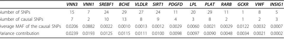
We examined the answers to the GAW17 simulation after our association analyses were completed. In the answers, Q2 is influenced by 72 SNPs in 13 genes, where the MAFs and effect sizes (b_i, the elements ofb) could be found for each causal SNP. Thus the variance contributed by each SNP to the phenotype could be cal-culated as 2 1q( −q)b_i2 under the assumption of an additive model, whereq is the MAF. Therefore we cal-culated the variance contribution for a gene using:

2 1 2

1

q_i q_i _i

i L

( − ) .

=

∑

b (7)

As shown in Table 1, both genes VNN3 and VNN1 have a variance contribution of approximately 0.02;

SREBF1,BCHE,VLDLR,SIRT1,PDGFD,LPL, and PLAT have variance contributions of approximately 0.01 indi-vidually; and RARB,GCKR,VWF, andINSIG1have var-iance contributions between 0.0002 and 0.005. The power is dependent on the variance attributed to the gene.

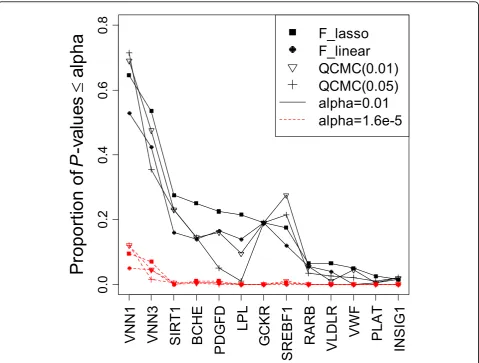
We evaluated the power of the four methods based on the 13 causal genes using the 200 replicates (Figure 1). In general, the LASSO regression outperformed linear regression for all causal genes and gained more than 10% power on the first four genes, as shown in Figure 1. The QCMC(0.01) method performed better than the QCMC(0.05) method because 91.7% of the MAFs of causal SNPs were less frequent than 0.01. Except for the

VNN1and SREBF1genes, the LASSO method was more

powerful than the two QCMC methods. This is quite easy to understand. The VNN1 gene has two causal SNPs, which have MAFs of 0.006 and 0.17, and all the causal SNP variants are less frequent than 0.005 in the

SREBF1 gene. For this reason, both the QCMC(0.01) and the QCMC(0.05) tests are able to collapse the cau-sal SNPs perfectly and thereby lead to a higher power than the LASSO approach for these two genes.

In general, all the tests increased the power when a gene’s contribution to the phenotype variation increased. However, we observed some exceptions, possibly because the power depends on many other factors, such as allele frequency and linkage disequilibrium among the SNPs within a gene. First, although their contribu-tions to the phenotype variation were similar, we had more power to detectVNN1, which consists of two cau-sal SNPs, with one of them being common (MAF = 0.17), than VNN3, which consists of seven rare causal SNPs. Second, for the GCKRgene, which has only one causal SNP, we also had reasonable power, in contrast to its small contribution to the phenotype variation. The association for these two genes was concentrated in a small number of causal SNPs and hence was easier to detect. Third, theSIRT1 andVLDLRgenes had a similar number of SNPs, number of causal SNPs, MAFs, and variance contribution; however, SIRT1 gained much more power thanVLDLR did. To understand why, we examined the linkage disequilibrium among each of these genes (using Haploview, http://www.broad.mit. edu/mpg/haploview) (Figure 2). SIRT1includes a com-mon SNP, C10S3059 (MAF = 0.167), that is in linkage disequilibrium with the causal rare SNP, C10S3048 (MAF = 0.002). The four gametes formed by these two SNPs are CT (83.7%), CC (16.6%), GC (0.1%), and GT (0.1%); and theD′value is 0.5 (R2 = 0.003). Among the 55 significant tests of the SIRT1gene in 200 replicates, 81.8%, 60%, and 50.9% of the LASSO models selected SNP C10S3059, C10S3048, or both, respectively, in their M1 models. However, for VLDLR, although SNP C9S341 (MAF = 0.095) was also in linkage disequili-brium with the causal SNP C9S444, which has MAF = 0.001 (D′= 0.384 and R2 = 0.002), it was not as com-mon as C10S3059 and the linkage disequilibrium pat-tern was not the same as that forSIRT1.

We also investigated the false-positive rates by count-ing the frequency of theP-values that were not larger

Table 1 True variance contributions of 13 causal genes given in the GAW17 answers

VNN3 VNN1 SREBF1 BCHE VLDLR SIRT1 PDGFD LPL PLAT RARB GCKR VWF INSIG1

Number of SNPs 15 7 24 29 27 24 11 20 29 11 1 8 5

Number of causal SNPs 7 2 10 13 8 9 4 3 8 2 1 2 3

(4)

0.

0

.2

0.

4

0.

6

0.

8

P

ropor

tion of

P

-v

al

ue

s

d

al

p

h

a

V

NN1

V

NN3

SI

R

T

1

BC

H

E

PD

G

F

D

LP

L

GC

K

R

SR

EBF

1

RA

RB

VL

D

L

R

VWF

PL

AT

INS

IG

1

F_lasso

F_linear

QCMC(0.01)

QCMC(0.05)

alpha=0.01

alpha=1.6e-5

Figure 1Power to detect 13 causal genes at the significance levels of 0.01 and 1.6 × 10–5in 200 replicates.Thex-axis indicates the 13 genes sorted in decreasing order of the power of theFLASSOtest, and they-axis indicates the corresponding power. The power is shown as solid black lines for the significance level 0.01 and as red dashed lines for the significance 1.6 × 10–5.

SIRT1

VLDLR

(5)

than a specific significance level for all of the 3,192 non-causal genes over the 200 replicates (Table 2). For some unknown reason, all four methods had inflated false-positive rates, and the inflation of the FLASSOtest was slightly bigger than that of the other three tests, but not significantly so.

Discussion and conclusions

In this study, we used the LASSO regression and calcu-lated the GDF for the F tests to avoid selection bias. This method requires using a parametric bootstrap to obtain the GDF; therefore it is computationally not as fast as the linear regression and collapsing methods. In general, theFLASSOtest is more powerful than the other methods.

Linear regression is the least powerful approach because of the large number of rare SNPs and because no deduction is made in the large number of degrees of freedom. The collapsing test requires specifying the pre-defined allele frequency threshold for grouping rare SNPs. It is difficult to determine this criterion optimally when in reality the true disease model is never known. For an extreme example, the QCMC(0.001) test was identical to the linear regression approach and the QCMC(0.1) test had no power at all in these data. Therefore, from this point of view, we recommend the LASSO approach for detecting rare SNPs.

Based on the power comparison of the SIRT1 and

VLDLRgenes, we observed some evidence that linkage disequilibrium played a significant role in detecting rare causal SNPs. If a rare causal SNP is in strong linkage disequilibrium with a common marker in the same gene, it will perform much better in terms of power. It would be of interest to further investigate the role of linkage disequilibrium between common noncausal mar-kers and rare causal SNPs on the power to detect rare causal SNPs and hence determine a more powerful test.

Acknowledgments

This work was supported by National Institutes of Health (NIH) grants HL074166, HL086718 from the National Heart, Lung, and Blood Institute, HG003054 from the National Human Genome Research Institute, RR03655 from the National Center for Research Resources, and P30 CAD43703 from the National Cancer Institute. The Genetic Analysis Workshops are supported by NIH grant R01 GM031575 from the National Institute of General Medical Sciences. This work was also partially supported by National Natural Science Foundation of China grant 10901031.

This article has been published as part ofBMC ProceedingsVolume 5 Supplement 9, 2011: Genetic Analysis Workshop 17. The full contents of the supplement are available online at http://www.biomedcentral.com/1753-6561/5?issue=S9.

Author details 1

Department of Epidemiology and Biostatistics, Case Western Reserve University, 10900 Euclid Ave, Cleveland, OH 44106, USA.2_{Key Laboratory for} Applied Statistics of MOE and School of Mathematics and Statistics, Northeast Normal University, Changchun 130024, China.

Authors’contributions

WG carried out the data analysis and drafted the manuscript. RCE and XZ participated in the design of the study and coordination and edited the manuscript. All authors read and approved the final manuscript.

Competing interests

The authors declare that there are no competing interests.

Published: 29 November 2011

References

1. Li B, Leal SM:Methods for detecting associations with rare variants for common diseases: application to analysis of sequence data.Am J Hum Genet2008,83:311-321.

2. Madsen BE, Browning SR:A groupwise association test for rare mutations using a weighted sum statistic.PLoS Genet2009,5:e1000384.

3. Price AL, Kryukov GV, de Bakker PI, Purcell SM, Staples J, Wei LJ, Sunyaev SR:

Pooled association tests for rare variants in exon-resequencing studies.

Am J Hum Genet2010,86:832-838.

4. Zhu X, Feng T, Li Y, Lu Q, Elston RC:Detecting rare variants for complex traits using family and unrelated data.Genet Epidemiol2010,34:171-187. 5. Guo W, Lin S:Generalized linear modeling with regularization for

detecting common disease rare haplotype association.Genet Epidemiol 2009,33:308-316.

6. Zhou H, Sehl ME, Sinsheimer JS, Lange K:Association screening of common and rare genetic variants by penalized regression.

Bioinformatics2010,26:2375-2382.

7. Tibshirani R:Regression shrinkage and selection via the LASSO.J R Stat Soc B1996,58:267-288.

8. Ye J:On measuring and correcting the effects of data mining and model selection.J Am Stat Assoc1998,93:120-131.

9. Li Y, Sung WK, Liu JJ:Association mapping via regularized regression analysis of single-nucleotide-polymorphism haplotypes in variable-sized sliding windows.Am J Hum Genet2007,80:705-715.

doi:10.1186/1753-6561-5-S9-S12

Cite this article as:Guoet al.:Evaluation of a LASSO regression approach on the unrelated samples of Genetic Analysis Workshop 17.

BMC Proceedings20115(Suppl 9):S12.