1752
Multi Objective Optimization of WEDM Process
Parameters Using Hybrid RSM-GRA-FIS, GA and SA
Approach
1
Bibhuti Bhusan Sahoo, 2Abhishek Barua, 3Siddharth Jeet, 4Dilip Kumar Bagal
1
Department of Mechanical Engineering,
Indira Gandhi Institute of Technology, Sarang, Dhenkanal, Odisha, 759146, India 2,3
Department of Mechanical Engineering,
Centre for Advanced Post Graduate Studies, BPUT, Rourkela, Odisha, 769004, India. 4
Department of Mechanical Engineering,
Government College of Engineering, Kalahandi, Bhawanipatna, Odisha, 766002, India Email:[email protected], [email protected]2, [email protected]3,
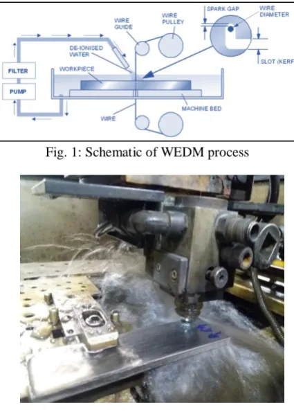
Abstract-Wire electric discharge machine (WEDM) is a thermo-electric spark erosion machining opearation employed for cutting very tough conductive material by means of the aid of a wire electrode. This paper presents a study that investigates the effect of the WEDM process parameters on the surface roughness and the kerf width of the stainless steel graded SS 304. Fifteen experimental runs carried out by based on Box-Behnken method of Response surface methodology (RSM) and fuzzy based grey relational analysis method is afterward used to find out an optimal WEDM parameter setting. Surface roughness, kerf width and tool wear rate (TWR) are considered as the quality responses. An optimal parameter setting of the WEDM process is obtained using Fuzzy based Grey relational analysis. By examining the Fuzzy-Grey relational grade matrix, the degree of influence for each controllable process parameter onto individual quality responses can be established. The pulse ON time is found to be the most influential factor for surface roughness, kerf width and tool wear rate. Genetic algorithm and Simulated annealing is used to calculate the best individual parameters along with the forecasted fitness values. It was found that every optimization techniques give similar factor setting.
Index Terms-WEDM, RSM, Fuzzy, Grey Relational Analysis, Genetic Algorithm, Simulated Annealing.
1. INTRODUCTION
Stainless steel is one of the extensively preferred materials for innumerable products which are often prepared by several cutting and finishing processes. Paid to the inherent characteristics of stainless steel such as high strength, rigidity and good corrosion resistance, its machinability is poor and it often requires high speed for machining. Additionally, the excellence of the machined surface is also moderately not up to the mark. Non-conventional machining methods such as WEDM have the prospective to machine stainless steel precisely. However, it is significant to select optimum arrangement of WEDM parameters for achieving optimal machining performance [1].
The most essential performance measures in WEDM are material removal rate (MRR), tool wear rate, surface roughness and kerf width. Discharge current, pulse duration, pulse frequency, wire speed, wire tension, average working voltage and dielectric flushing conditions are the machining parameters which influence the performance measures. Among the other performance measures, the kerf width, which evaluates the dimensional accuracy of the finished part, is of utmost importance. In WEDM operations, surface roughness is one of the components that
describe the surface integrity. In setting the machining parameters, the main objective is the least amount of surface roughness with the minimum kerf width. In past, a lot of work has been carried out to investigate the effect of WEDM parameters on various performance parameters [1].
Keeping this in view, the present work is aimed to investigate the effect of three WEDM parameters (current, pulse ON time and pulse OFF time) on surface roughness, kerf width and tool wear rate during WEDM of SS [3]. The RSM Box-Behnken design is used for experimental planning for this purpose. Hybrid Fuzzy based Grey relational analysis is then applied to study how the input factors influence the quality targets of surface roughness, kerf width and tool wear rate. Through analyzing the Fuzzy-Grey relational grade matrix, the most influential factors for individual quality responses of cutting operations can be identified. Further Genetic Algorithm and Simulated Annealing is also used for obtaining optimum factor setting.
2. MATERIAL USED AND EXPERIMENTAL SETUP
1753 composition of the work-piece material is shown in
Table 1.
Table1: Material composition of stainless steel
Element Concentration
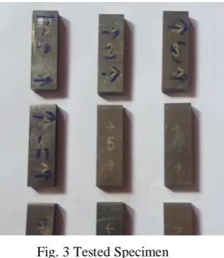
The experimental studies were performed on Electronica Group Ecocut travelling WEDM machine. This machine can be utilized to cut work piece in accordance with the fixed locus. Different settings of current, pulse ON time and pulse OFF time are taken in the experiments. Frequency setting is retained fix throughout the experiments.
Fig. 1: Schematic of WEDM process
Fig. 2 Work Table
Table 2: Input Variables with Levels value
3. EXPERIMENTAL DESIGN WITH RESPONSE SURFACE METHOD
Response surface method is a collected works of mathematical and statistical techniques that are compliant for modeling and analysis of problems in which response is partial by several input parameters, and the main objective is to get the correlation between the response and the variables inspected. Response surface method has many advantages and has effectively been used to study and optimize the process parameters. It gives mammoth information from a small number of experiments [4]. In addition, it is possible to distinguish the interaction effect of the independent parameters on the response. The model easily illuminates the effect for binary combination of the independent process variables. Furthermore, the empirical model that associated the response to the independent variables is used to acquire information. RSM has been widely utilized in investigating various processes, designing the experiment, building models, evaluating the effects of several factors and finding for optimum conditions to suggest desirable responses and reduce the number of experiments. The experimental values are analyzed, and the mathematical model is then developed that illustrates the relationship between the process variable and response [2]. The following
where Y is the corresponding response, Xi is the input
variables and Xii and XiXj are the squares and
1754
3.1. Grey Relational Analysis
The grey relational analysis is really an extent of the absolute value of data difference between the sequences, and can be utilized for estimation of the correlation between the sequences. The following sections present the practice for grey relational analysis that has been used [12].
3.1.1. Data pre-processing
Data pre-processing is utilized to transfigure the given data order into dimensionless data categorization and it incorporates the transfer of the original sequence to a comparable sequence. Let the original reference sequence and comparability arrangement be represented as and , i = 1, 2,…, m; t = 1, 2,…n respectively, where m is the total number of experiment to be taken, and n is the total number of observation data. Data pre-processing translates the original sequence to an equivalent sequence. Several approaches of pre-processing data can be used in Grey relation analysis, depending on the features of the original sequence. For “Larger the better”, if the target value of original sequence is infinitely large then the normalized experimental results can be described as-
(ii)
For “Smaller the better”, when the target value of original reference sequence is infinitely small then the normalized results is expressed as-
(iii)
For “Nominal the best”, if a defined target value j exists, when the target value is closer to desired value the normalization is done as-
(iv)
3.1.2. Grey relational coefficients and Grey relational grades
After the data pre-processing, a grey relational coefficient is calculated by means of the pre-processed sequences. The grey relational coefficient can be calculated as-
and 0
< 1 (v)
After calculation of the grey relational coefficients, grey relational grade is calculated using the following equation- comparability sequences. In case of two indistinct sequences, the grey relational grade is equal to 1. The grey relational grade also stipulates the degree of influence applied by the comparability sequence on the reference sequence. Consequently, if a particular comparative sequence is more significant to the reference sequence than other comparability sequences, the grey relational grade for that comparability sequence and the reference sequence will surpass as compared to other grey relational grades [12].
3.2. Fuzzy inference system
Fuzzy inference or fuzzy ruled based system organizes four representations; fuzzification interface, rule base and database, decision making unit and lastly a defuzzification interface. Membership functions of the fuzzy sets are delineated by the database, which are employed in fuzzy rules, inference operation of the outlined rules is proficient by the decision making unit. Translations of inputs into degrees of match with etymological values are carried out by fuzzification interface; defuzzification interface translates the fuzzy results of the inference into crisp output [6]. The fuzzy rule base is determined by if‐then control rules with atleast two inputs and one output for example.,
Rule 1: if x1 is A1 and x2 is B1 then y is C1 else
1755 Fig. 3Fuzzy editors on Fuzzy inference system
3.3. Genetic Algorithm
Genetic Algorithm is based on the biological evolution process which is used to evolve solutions to complex optimization problems. A possible solution to a problem may be represented by a set of parameters well-known as genes. These genes are combined together to form a string which is referred to as a chromosome. The set of constraints represented by a particular chromosome is called as genotype. This genotype contains the information obligatory to construct an organism called the phenotype. A fitness function is analogous to the objective function in an optimization problem. The fitness function returns a single numerical fitness which is proportional to the utility or the ability of the individual which that chromosome represents. Two parents are selected and their chromosomes are recombined, typically using the mechanisms of crossover and mutation. Crossover is more important for rapidly exploring a search space. Mutation provides only a small amount of random search [11].
3.3.1. Algorithm of GA approach
1. Generate random population of chromosomes. 2. Evaluate the fitness of each chromosome in the population.
3. If the end condition is fulfilled, stop and return the best solution in current population.
4. Create a new population by repeating the following steps until the new population is complete. Select two parent chromosomes of the population according to their fitness. With a crossover probability, cross over
5. Replace: Use new generated population for a further run of the algorithm.
6. Go to step 2.
3.4. Simulated annealing
Simulated Annealing is a probabilistic method which emulates the process of annealing (slow cooling of
molten metal) in order to achieve minimum unguent value in a minimization problem. The cooling phenomenon is conceded out by governing a temperature like parameter presented with the concept of the Boltzmann probability distribution [10]. Deliberating to this dispersal a system in thermal equilibrium at temperature T has its energy probabilistically dispersed as per Equation (vi).
P(E) = exp(−ΔE/kT) (vii)
Where the exponential term is Boltzmann coefficient and k is the Boltzmann constant. According to thesurface roughness tester (model: Mitutoyo SurfaceRoughness Tester SJ – 400). The stereo-zoom microscope (make: Focus, Japan) was used to get kerf width values and tool wear rate was measured using Scanning Electron Microscope.
4. RESULTS AND DISCUSSION
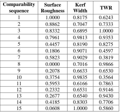
The samples are cut into desired size by using WEDM which is shown in fig 4.
Fig. 3 Tested Specimen
1756 the reference sequence , t = 1, 2. Moreover, the
results of fifteen experiments were the comparability sequences , i = 1, 2, ...,15, t = 1, 2. Table 4 listed all of the sequences after implementing the data pre-processing using Eq. (iv). The references and the
comparability sequences were denoted as and
, respectively. Also, the deviation sequences , , and (t) for i = 1, 2, ..., 15, t = 1, 2 can be calculated.
Table 3: RSM based Box-Behnken design for experimental runs and responses
Run
No. A B C
Surface Roughness
(μm)
Kerf Width (μm)
TWR (g/min3)
1 1.0 6 2 2.311 194.609 4.6
2 2.0 6 2 2.575 205.279 3.64
3 1.0 8 2 2.698 206.718 1.29
4 2.0 8 2 2.784 179.122 1.86
5 1.0 7 1 3.597 194.47 2.81
6 2.0 7 1 4.212 179.47 6.05
7 1.0 7 3 3.28 186.533 10.1
8 2.0 7 3 4.631 205.57 5.9
9 1.5 6 1 4.149 209.192 7.05
10 1.5 8 1 3.76 271.93 6.96
11 1.5 6 3 3.25 213.61 2.33
12 1.5 8 3 4.09 210.16 2.09
13 1.5 7 2 4.01 210.07 1.78
14 1.5 7 2 3.66 193.4 5.9
15 1.5 7 2 4.49 177.35 4.3
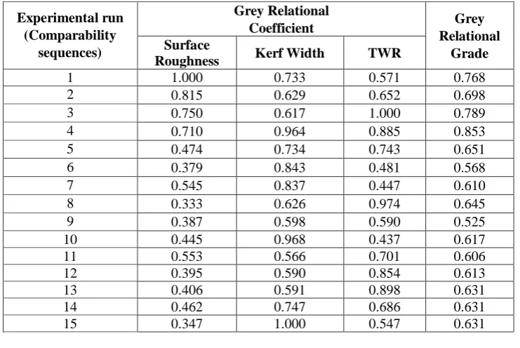
The distinctive coefficient can be substituted for the grey relational coefficient in Eq. (v). If all the process parameters have equivalent weighting, is set to be 0.5. Table 5 gives the grey relational coefficients and the grade for all fifteen comparability sequences. This investigation employs the response table of the Response Surface method to calculate the average Grey relational grades for each factor level, as illustrated in Table 5.
Table 4: The sequence after data pre-processing
Comparability sequence
Surface Roughness
Kerf
Width TWR
1757 Table 5: Grey relational coefficient and grey relational grade for fifteen comparability sequences.
Experimental run (Comparability
sequences)
Grey Relational
Coefficient Grey
Relational Grade Surface
Roughness Kerf Width TWR
1 1.000 0.733 0.571 0.768
2 0.815 0.629 0.652 0.698
3 0.750 0.617 1.000 0.789
4 0.710 0.964 0.885 0.853
5 0.474 0.734 0.743 0.651
6 0.379 0.843 0.481 0.568
7 0.545 0.837 0.447 0.610
8 0.333 0.626 0.974 0.645
9 0.387 0.598 0.590 0.525
10 0.445 0.968 0.437 0.617
11 0.553 0.566 0.701 0.606
12 0.395 0.590 0.854 0.613
13 0.406 0.591 0.898 0.631
14 0.462 0.747 0.686 0.631
15 0.347 1.000 0.547 0.631
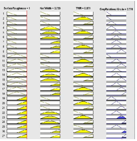
The fuzzy logic approach is performed to a single grey‐fuzzy reasoning grade than considering complicated multiple outputs. Mamdani’s inference method is chosen from different techniques available for obtaining membership function values and centroid method is used for defuzzification approach. The fuzzy logic technique produces an improved lesser uncertain grey‐fuzzy relational grade than the normal grey relational approach, providing a greater value of the grey‐fuzzy reasoning grade with a reduction in the fuzziness of data’s. For fuzzifying grey relational coefficient of each response, fuzzy rules and triangular membership function as Low, Medium and High are established. To formulate the statement for prediction fuzzy logic, If‐Then rule statements are used, which have three grey relational coefficients such as surface roughness, kerf width and TWR with one output as a grey‐fuzzy reasoning grade. The fuzzy subsets that are applied to the multi‐response output and the fuzzy subset ranges are presented in Table 6. Fuzzy logic tool in MATLAB software is used for this grey‐fuzzy technique. The grey‐fuzzy output is segregated into five membership functions. For activating the fuzzy inference system (FIS) a set of rules are written and to predict the reasoning grade FIS is evaluated for all the 15 experiments. Fig. 6 shows the rule editor in fuzzy environment for predicting the grey‐fuzzy reasoning
grade, for a given input value of GRC value of surface roughness, kerf width and TWR.
Table 6: Range of fuzzy subsets for grey‐fuzzy reasoning grade (Triangular Membership Function)
Range of Value Conditions
[-0.25 0 0.25] Very Low [0 0.25 0.5] Low [0.25 0.5 0.75] Medium
[0.5 0.75 1] High [0.75 1 1.25] Very High
1758 Fig. 6 Rule editors in fuzzy environment
Table 7: Grey‐fuzzy reasoning grade
Sl No.
Grey Relational
Grade
Grey-Fuzzy Reasoning
Grade
% Improvement
1. 0.768 0.778 1.32
2. 0.698 0.665 -4.79 3. 0.789 0.782 -0.88
4. 0.853 0.869 1.85
5. 0.651 0.652 0.21
6. 0.568 0.647 13.99
7. 0.610 0.662 8.56
8. 0.645 0.668 3.64
9. 0.525 0.567 8.01
10. 0.617 0.678 9.95 11. 0.606 0.609 0.43 12. 0.613 0.673 9.78 13. 0.631 0.694 9.90 14. 0.631 0.644 1.98 15. 0.631 0.667 5.62
Since, the Grey fuzzy Reasoning Grade represents the level of correlation between the reference and the comparability sequences, the larger Grey relational grade means the comparability sequence exhibiting a stronger correlation with the reference sequence. Based on this study, one can select a combination of the levels that provide the smaller average response. In Fig. 7, the combination of A2 B1 and C1 shows the
smallest value of the Mean effect plot for the factors A, B and C respectively. Therefore, A2B1C1 i.e.
current of 1.5amp, pulse on time of 6 μs and pulse off time of 1 μs is the optimal parameter combination.
Fig. 7: Main effect plot with factors and their levels
Fig. 8: Residual Plots for Grey‐fuzzy reasoning grade
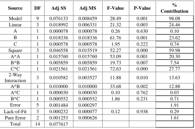
1759 Table 8: ANOVA result for Grey fuzzy Reasoning Grade
Source DF Adj SS Adj MS F-Value P-Value % Contribution
Model 9 0.076133 0.008459 28.49 0.001 98.08 Linear 3 0.018992 0.006331 21.32 0.003 24.46 A 1 0.000078 0.000078 0.26 0.630 0.10 B 1 0.018336 0.018336 61.76 0.001 23.62 C 1 0.000578 0.000578 1.95 0.222 0.74 Square 3 0.046558 0.015519 52.27 0.000 59.98
A*A 1 0.015760 0.015760 53.09 0.001 20.30 B*B 1 0.005859 0.005859 19.73 0.007 7.54 C*C 1 0.021561 0.021561 72.63 0.000 27.77 2-Way
Interaction 3 0.010582 0.003527 11.88 0.010 13.63 A*B 1 0.010000 0.010000 33.68 0.002 12.88 A*C 1 0.000030 0.000030 0.10 0.762 0.03 B*C 1 0.000552 0.000552 1.86 0.231 0.71
Error 5 0.001484 0.000297 1.91
Lack-of-Fit 3 0.000232 0.000077 0.12 0.938 0.29 Pure Error 2 0.001253 0.000626 1.61
Total 14 0.077617
S=0.0172303, R-sq=98.09%, R-sq(adj)=94.65%, R-sq(pred)=91.59%
4.1 Optimization using genetic algorithm and simulated annealing
The selection of optimum parameters has always been a complex task in designing. In practice, the designing parameters are mostly selected on the basis of human judgment, experience and referring the available catalogues and handbooks which leads to non-optimal parameters. The optimum parameters can be achieved efficiently by using asuitable optimization method. Therefore, the designing parameters are defined in the regular optimal format and solved using genetic algorithm and simulated annealing. The minimization problem formulated in the standard mathematical format is as below:
Minimize
3.462-1.501a-0.636b+0.3882c+0.2613a2+0.03983b2 -0.07642c2+0.1000ab+0.0055ac-0.01175bc (viii) Subjected to constraints:
1 ≤ a ≤ 2 6 ≤ b ≤ 8 1 ≤ b ≤ 3
Genetic algorithm and simulated annealing was utilized to solve the above objective function. For GA, a population size of 200 and initial population range covering the entire range of values for a and b has
been used to avoid getting local minimum. The cross over rate used was 0.8 and mutation function was
uniform. The scaling function and selection function were rank and uniform respectively. The optimum parameters obtained by the GA are shown in Figure 9. The optimal solution was found out after 86 generations.
1760 Fig. 9 variations of the best fitness value with generations and the optimum parameters using GA
Fig. 10 variations of best fitness value with generations and the optimum parameters using SA
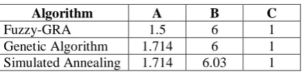
Table 9: Optimal cut parameters using three optimization methods
Algorithm A B C
Fuzzy-GRA 1.5 6 1
Genetic Algorithm 1.714 6 1 Simulated Annealing 1.714 6.03 1
5. CONCLUSION
The properties of input parameters i.e. current, pulse ON time and pulse OFF time are experimentally studied throughout machining of SS 304 using WEDM process. The fuzzy-grey relational analysis based on the RSM table was used to optimize the WEDM process parameters. Based on the outcomes of the present study, the following inferences are shown:
Surface roughness, kerf width and tool wear rate increases when the pulse ON time leads to increase.
From ANOVA analysis, the percentage of contribution to the WEDM process, in sequence is found out to be the pulse ON time, the current and the pulse OFF time. Hence, the pulse ON time is the most important controlled parameter for the WEDM practice when minimization of the surface roughness, kerf width and tool wear rate are concurrently considered.
1761 circularity, cylindricity, machining cost etc are can be
considered for future research in WEDM process. More reliable prediction of unit process will enable industry to develop more optimal values during selection of machining parameters for WEDM.
Acknowledgments
The Authors would like to thank all technical assistant of central workshop and Principal of Government College of Engineering Kalahandi, Bhawanipatna, Odisha for aiding and helping in preparation specimen and National Institute of Technology, Rourkela, Odisha for machining and measurement process for completion of this research.
REFERENCES
[1] Khan, Z. A.; Siddiquee, A. N.; Khan N. Z.; Khan U.; Quadir, G. A. (2014): Multi response optimization of Wire electrical discharge machining process parameters using Taguchi based Grey Relational Analysis. Procedia Materials Science, 6, pp. 1683 – 1695.
[2] Sharma, N.; Singh, A.; Sharma, R.; Deepak (2014) Modelling the WEDM Process Parameters for Cryogenic Treated D-2 Tool Steel by integrated RSM and GA. Procedia Engineering, 97, pp. 1609 – 1617.
[3] Senthil, P.; Vinodh S.; Singh, A. K. (2014): Parametric optimisation of EDM on Al-Cu/TiB2 in-situ metal matrix composites using TOPSIS method. Int. J. Machining and Machinability of Materials, 16(1).
[4] Pradhan, M. K. (2018): Optimisation of EDM process for MRR, TWR and Radial overcut of D2 steel: A hybrid RSM-GRA and Entropy weight based TOPSIS Approach. Int. J. Industrial and Systems Engineering, 29(3), pp. 273-302.
[5] Mahapatra S. S.; Patnaik, A. (2007): Optimization of wire electrical discharge machining (WEDM) process parameters using Taguchi method. Int J Adv Manuf Technol, 34, pp. 911–925.
[6] Senthilkumar, N.; Sudha, J.; Muthukumar, V. (2015): A grey‐fuzzy approach for optimizing machining parameters and the approach angle in turning AISI 1045 steel. Advances in Production Engineering & Management, 10(4), pp. 195–208. [7] Yang, S. H.; Srinivas, J.; Mohan, S.; Lee, D. M.;
Balaji, S. (2009): Optimization of electric discharge machining using simulated annealing. Journal of Materials Processing Technology, 209, pp. 4471–4475.
[8] Santhanakumar, M.; Adalarasan, R.; Raj, S. S.; Rajmohan, M. (2017): An integrated approach of TOPSIS and response surface methodology for optimising the micro WEDM parameters. Int. J. Operational Research, 28(1).
[9] Zhang, G.; Zhang, Z.; Guo, J.; Ming, W.; Li, M.; Huang, Y.; (2013): Modeling and Optimization of Medium-Speed WEDM Process Parameters for Machining SKD11. Materials and Manufacturing Processes, 28, pp. 1124–1132.
[10]Kolahan, F.; Golmezerji, R.; Moghaddam, M. A. (2012) Multi Objective Optimization of Turning Process using Grey Relational Analysis and Simulated Annealing Algorithm. Applied Mechanics and Materials, 10-116, pp. 2926-2932. [11]Sangwan, K. S.; Kant, G. (2017): Optimization of
Machining Parameters for Improving Energy Efficiency using Integrated Response Surface Methodology and Genetic Algorithm Approach. Procedia CIRP, 61, pp. 517 – 522.