Performance Evaluation Bulk Arrival and Bulk Service with Multi Server using Queue Model

(1)

3718

Performance Evaluation Bulk Arrival and Bulk

Service with Multi Server using Queue Model

Jitendra Kumar

1

and Vikas Shinde

2

1,2_{Department of Applied Mathematics}

Madhav Institute of Technology & Science, Gwalior, (M. P.) INDIA E-mail: [email protected] , [email protected]

Abstract- This paper deal bulk arrival and bulk service queueing model. Arrival and service rate is considered in batch size α and β respectively for multi-server model. Performance measure have been carried out viz average number of customers in the queue, average number of customers in the system, average waiting time of customers in queue, average waiting time of customers in the system, response time and efficiency of the server corresponding to customers. Numerical illustrations have been provided to validate our results.

Index Terms - Bulk arrival, Bulk service, Multi-servers queue model and Transient states.

1. INTRODUCTION

In manufacturing process the work-pieces arrive at a centre in batches and they leave in batches. A batch consists of identical work-pieces that are processed and then transported in batches for further processing. Such a situation can be modeled as queues with bulk arrivals. There is a discipline within the mathematical theory of probability, called a bulk queue (also called batch queue). Various researchers have been focused such issues in dimension. Pang and Whitt [1] motivated by large-scale service systems, and considered an infinite-server queue with batch arrivals, where the service times are dependent within each batch. Zwart et al. [2] examined the existing modal, the dependent between queueing time and wait – to – batch time has been identified. Khalaf et al. [3]

introduced four different main servers with

interruptions and a stand-by. Bagyam et al. [4] considered bulk arrival general service retrial queueing system where server provides two phases of service-essential and optimal. After each service completion, the server searches for customers in the orbit. Customers may balk or renege at particular times and accidental and active breakdown of the server. Chen et al. [5] Markovian bulk-arrival and bulk service queue incorporating state-dependent control and obtain the behavior of queue length regarding to hitting and busy period are also explored. Ghimire et al. [6] formulated mathematical model with the balk queueing model with fixed batch size, and also obtained mean waiting time and mean time spent in the system and queue. Briere and Chaudhry [7] and Kambo and Chaudhry [11] used numerical approaches to get the performance indices. Chaudhry and

Templeton [8] gave more extensive study on batch arrival/service queues. Downton [10] derived the relation between limiting queue size distributions at arrival and departure epochs. Dragovic et al. [12]

Developed this modeled by MX/M/n/m queue with

finite waiting areas and identical and independent cargo-handling capacities. Gupta and Goswani [13] analyzed a discrete-time infinite buffer bulk-service. Some analytic computational results for discrete-time bulk service queue have been reported. Gupta et al. [14] have discussed the same queueing model for EAS and LAS- DA, and developed a recursive procedure to obtain system length distribution at pervasive arbitrary and outside observer’s observation epochs. Kumar et al. [15] proposed various performance indices for multi-server model.

We organized this paper as follows. Section 2 & 3 presented the mathematical notations and model of the queueing system. In section, 4 described mathematical models corresponding to queue system. Performance measure as average number of customers in the queue, average number of customers in the system, average waiting time of customers in the queue and average waiting time of customers in the system is obtained in section 5. In section 6, numerical illustration and graphical representation have been drawn and finally Section, 7 conclude the paper.

2. NOTATION

n = Number of customers in the system λ = Arrival rate

α = Customers in Group or Batch (as different size) for arrival rate

(2)

3719 β = Customers in Group or Batch (as different size)

for service rate

c = Serving rate when c > 1 in a system

ρ=System intensity or utilization factor (ρ= αλ / βcμ) Lq = Average number of customers in the queue Ls = Average number of customers in the system Wq =Average waiting time of customers in the

queue

Ws =Average waiting time of customers in the system

Es = Efficiency of the system

3. MODEL DESCRIPTION

Different structures of queueing model have been discussed. Customers requiring services are generated over time by an input source. This service mechanism is described in two ways:

 Single queue with multiple server model

 Multiple queue with multiple server model

Arrival Rate

Queue

Departure Rate

Server 1

Server 2

Server C

No. of Customers

Figure 1: Queuing Model for Single-Queue with Multiple Parallel Servers

Arrival Rate

Queue 2

Departure Rate

Server 1

Figure2: Queuing Model for Multi Queues with Multiple Parallel Servers

We are discussing two types queue system multi queue and multi queue with multi servers are illustrated in figures 1 & 2.

4. MATHEMATICAL MODEL

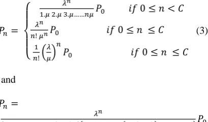
In Mα|Mβ|C queue model, the arrival rate remains

same as M|M|1 queues but the service rate will depend

on the number of servers. The service rate will be nμ

Figure 3 Steady –state diagram

If there is a single server, mean service rate μn = μ for

all n. but there are c servers working independently of each other. Therefore, over all service rate, when there are n customers in the system, may be obtain two situations

(i) If n< C, all the customers may be served

simultaneously and there will be no queue. Hence (C - n) number of servers may remain idle and

(b) The average service rate

{

(c) The average arrival rate is less than c μ i.e., λ/cμ.

We have for Poisson queue system,

Substituting the assumption (a) and (b) in (1) we get

(3)

3720

5. PERFORMANCE MEASURES OF Mα|Mβ|C QUEUING MODEL customers in the system. Also, obtain average number of idle servers corresponding to customers and efficiency of system with queue model with utilization factor. All these mathematical expressions of this queue model are termed as the performance evaluate of the system and described as follows:

5.1 Average number of customers in the queue :

5.5 Average Response time : (Rt)

( )

Where C(c, λ/μ) is the probability that an arrival customer is forced to join the (all servers are occupied), referred to as Erlang’s C formula

( )

5.6 Efficiency of system with queue model : (Es)

Special Cases:

In this section, we described two special cases

Mα/ M/1 and M/Mβ/1. If

(i) Mα/ M/1 (see Ref. 17)

(ii)M/Mβ/1 (see Ref. 11)

6. NUMERICAL APPROACH AND GRAPHIC INTERPRETATIONS

(4)

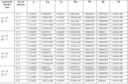
3721 Table 1 Performance measure response time, efficiency of server with utilization

Table 2 Performance measure response time, efficiency of server with utilization

Arrival & Service

rate

No. of Servers

ρ Lq Ls Wq Ws Rt Ef

α = 3 β =2

C= 2 0.974026 4.50567 5.4797 0.0300378 0.0365313 0.0095919 0.0273985 C= 3 0.649351 0.00961011 0.658961 9.61011e-005 0.00658961 0.0071067 0.0032948 C=4 0.487013 0.000149637 0.487163 1.99516e-006 0.0064955 0.00670674 0.00243581 C=5 0.38961 2.21601e-006 0.389613 3.69334e-008 0.00649354 0.00656627 0.00194806 C=6 0.324675 2.74828e-008 0.324675 5.49655e-010 0.00649351 0.0065137 0.00162338

α = 3 β = 4

C= 2 0.487013 0.0378565 0.524869 0.000504753 0.00699826 0.00874704 3.49913e-005 C= 3 0.324675 0.000505755 0.325181 1.01151e-005 0.00650362 0.00678301 3.25181e-005 C=4 0.243506 5.87626e-006 0.243512 1.567e-007 0.00649366 0.00653714 3.24683e-005 C=5 0.194805 5.30361e-008 0.194805 1.76787e-009 0.00649351 0.00649948 3.24675e-005 C=6 0.162338 3.70077e-010 0.162338 1.48031e-011 0.00649351 0.00649424 3.24675e-005

α = 3 β = 5

α = 3 β =8

C= 2 0.243506 0.00383723 0.247344 0.000102326 0.00659583 0.00733735 3.29792e-005 C= 3 0.162338 3.37642e-005 0.162371 1.35057e-006 0.00649486 0.00654691 3.24743e-005 C=4 0.121753 2.22009e-007 0.121753 1.18405e-008 0.00649352 0.00649744 3.24676e-005 C=5 0.0974026 1.07343e-009 0.0974026 7.15623e-011 0.0064935 0.00649378 3.24675e-005 C=6 0.0811688 3.91077e-012 0.0811688 3.12862e-013 0.00649351 0.00649352 3.24675e-005

Arrival & Service rate

α = 4 β = 3

α = 4 β =5

α = 4 β = 7

α = 4 β = 9

(5)

3722 Table 3 Performance measure response time, efficiency of server with utilization

Table 4 Performance measure response time, efficiency of server with utilization

Arrival & Service rate

α = 4 β = 3

α = 4 β =5

α = 4 β = 7

α = 4 β = 9

Arrival & Service

rate

α = 3 β =7

α = 5 β = 7

α = 6 β =7

α = 9 β =7

(6)

3723

Response time vs Efficiency of system with Utilization

Utilization

Respnse time & Efficiency of Server with Utilization

Utilization

Response time & Efficiency of Sever with Utilization

Utilization

Response time & Efficiency of Sever with Utilization

Number of Channel

Response time vs efficiency of system with Utilization

Utilization

Response time vs Efficiency of System with Utilization

Utilization

Response time vs Efficiency System with Utilization

(7)

3724

Utiliation

Response time vs Efficiency of System with Utilization

Utilization

Utilization1

Utilization Response time Efficiency of system

2 2.5 3 3.5 4 4.5 5 5.5 6

(8)

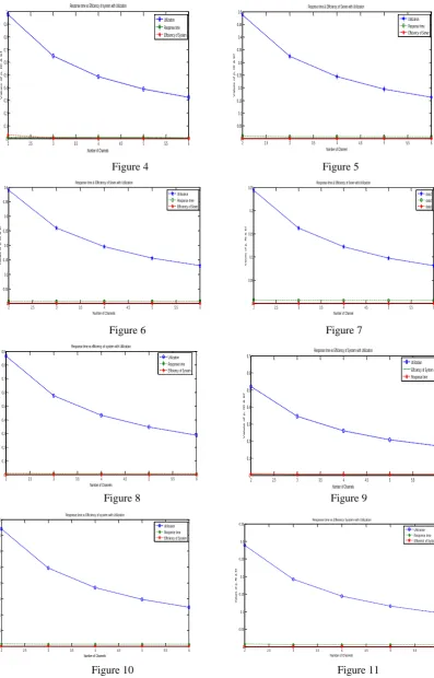
3725 Here, we represented the graphical interpretation

between response time vs efficiency of system (server) with utilization in figures 4 to 19 by varying various parameters of bulk arrival and bulk service with multiple number of servers. It has been observed that the performance of system (server) response time and utilization of system goes down when the number of channels increases.

7. CONCLUSION

In this paper, we obtained explicit mathematical formulae for real life problems such as customer’s dispatching strategies for bulk arrival and bulk service with multi-server which consist of some combination of customers with system holding and cancellation strategies. The numerical results have been carried out by using MATLAB-9. Result shows applicability in several real-world situations such as passport office, airport, manufacturing system, transportation system, assembly line system and other place in overall supply chain management systems. This model can be studied under the provision of time dependent arrival and service rate which make our model more realistic environment.

REFERENCES

[1] G. Pang and W. White “Infinite-Server Queues with Batch Arrivals and Dependent Service Times”, Probabulity in the Engineering and Informational Sciences, volume 26, pages 1-21, 2011.

[2] K. Wu, F. L. McGinnis and B. Zwart. “Approximating the performance of a batch

service queue the M/Mk/1 Model” IEEE

Transactions on Automation Science and Engineering, volume 8 (1), pages 95-102, 2011. [3] R. F. Khalaf and J. Alali. “Queueing Systems with Four Different Main Server’s Interruptions and a Stand-By Server”, International Journal of Statistics and Probability, volume 3, pages 49-54, 2014.

[4] J. E. A. Bagyam, K. U. Chandrika and K. P. Rani. “Bulk Arrival Two Phase Retrial Queueing System with Impatient Customers, Orbital Search, Active Breakdowns and Delayed Repair”, International Journal of Computer Applications, volume 73, pages 13-17, 2013. [5] A. Chan, P. Pellett, J. Li, and H. Zhang.

“Markovin bulk-arrival and bulk-service queue

with State- dependent control, Queueing

System”, volume 64, pages 267-307, DOI 10.1007/s11134-009-9162-5, 2010.

[6] S. Ghimire, R. P. Ghimire, and G. Hahadur.

Mathematical models of Mb/M/1 bulk arrival

Queueing System”, Journal of the Institute of Engineering, volume 10(1), pages 184-191, 2014.

[7] G. Briere and M. L. Chaudhry. “Computational analysis of single server bulk-service queues,

M/GB/1”, Advanced Applied Probability, volume

21, pages 207-225, 1989.

[8] M. L. Chaudhry and J.G.C. Templeto. “A First Course in Bulk Queues”, Wiley, New York, 1983.

[9] J. W. Cohen. “The Single Server Queue”, 2nd edition, North-Holland, Amsterdam, 1980. [10] F. Downton. “Waiting time in bulk Service

Queues”, Journal of Royal Statistical Society, B17, pages 256-261, 1955.

[11] N. S. Kambo and M. L. Chaudhry. “A single-server bulk-service queue with varying capacity and Erlang Input”, INFOR, volume. 23(2), pages 196-204, 1985.

[12] B. Dragovic, N.K. Park, M. D. Zrnic and R. Mestrovic. “Mathematical model of multi-server queueing system for dynamic performance evaluation in port” Mathematical Problems in Engineering, volume 2012, pages 1-19, 2012. [13] U. C. Gupta and V. Goswani. “Performance

analysis of finite buffer discrete time queue with bulk service”, Computers and Operation, volume 29, pages 1331-1341, 2002.

[14] U. C. Gupta, S. K. Samanta and R. K. Sharma. “Computing queueing length and waiting time distribution in finite discrete – time multi-server queue with late and delay arrivals”, Computers and Mathematics with Applications, volume 48, pages 1557-1578, 2004.

[15] J. Kumar, V. Shinde, B. B. Singh and A. Kumar. “Analysis of performance measure of multi-server based on queue length and waiting time”, Journal of Ganita Sandesh, volume 24(2), pages 127-134, 2010.