Automatic Biomedical Term Polysemy Detection
Juan Antonio Lossio-Ventura
1,2, Clement Jonquet
1,2, Mathieu Roche
1,2,3, Maguelonne Teisseire
1,4,5LIRMM1, University of Montpellier2, Cirad3, Irstea4, TETIS5 Montpellier, France
[email protected], [email protected], [email protected], [email protected]
Abstract
Polysemy is the capacity for a word to have multiple meanings. Polysemy detection is a first step for Word Sense Induction (WSI), which allows to find different meanings for a term. The polysemy detection is also important for information extraction (IE) systems. In addition, the polysemy detection is important for building/enriching terminologies and ontologies. In this paper, we present a novel approach to detect if a biomedical term is polysemic, with the long term goal of enriching biomedical ontologies. This approach is based on the extraction of new features. In this context we propose to extract features following two manners: (i) extracted directly from the text dataset, and (ii) from an induced graph. Our method obtains an Accuracy and F-Measure of 0.978.
Keywords:Polysemy Detection, Biomedical Polysemy Detection, BioNLP, Disambiguation, Classification
1.
Introduction
The Web is by far the largest information archive avail-able worldwide evolving. This resource contains impor-tant information about several domains. This is the case for biomedicine, that brings knowledge through numerous publications (El-Rab et al., 2013). In this context, there are several methods to extract relevant information tackling the disambiguation problem (El-Rab et al., 2013; Zhong and Ng, 2012). This issue has been also recently addressed by the research of concepts, analyzing text to extract in-stances of concepts associated with user queries (Agirre et al., 2014). The ontologies are very useful for the identi-fication of concepts; the main objective is the creation of knowledge in a domain. They must be regularly enriched by the introduction of new terms. So, to enrich ontolo-gies/vocabularies with new terms, it is necessary to know the possible senses of a term, this is the well known Word Sense Induction (WSI) domain. One preliminary step is to detect if a term is polysemic (binary decision). If the term is polysemic, then to make a deep search of their senses. To our knowledge, there are no studies for the same purpose.
Therefore, in order to meet the challenge, we propose a novel methodology to detect if a term is polysemic by defin-ing new features, extracted directly from the textual dataset and from an induced graph, as described after. In turn, our methodology uses two dictionaries allowing us to de-termine the use of a same term in different domains (i.e., biomedical and agronomy). To the best of our knowledge, graphs have never been used to define features for classifi-cation purpose. In this work the main idea is to capture the dataset characteristics from the structural shape and size of graph induced from the dataset. This approach enables to obtain excellent results, with 97.8% for Accuracy and F-Measure.
The paper is organized as follows. First, the methodology is detailed in Section 2.. Results are presented in Section 3.. We discuss related work in Section 4. followed by conclu-sion and perspective in Section 5..
2.
Towards Polysemy Detection
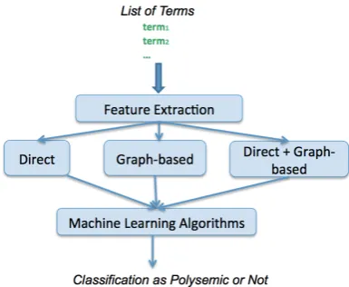
In this section, we present the proposed methodology to de-termine if a biomedical term is polysemic. We present the new features that serve to characterize the dataset. Figure 1 shows the workflow of our approach, which is described hereafter.
Figure 1:Workflow Methodology for Polysemy Prediction.
2.1.
Extraction of New Features
We present new features based on statistical measures to characterize our dataset. They are extracted directly from the dataset and from an induced graph. We select appro-priate learning algorithms to determine if a term is poly-semic. Totally 23 features are proposed, 11 direct and 12 from the induced graph. Their effectiveness are illustrated by comparing the results obtained by different supervised algorithms.
Notation: for each term t let At = ai the set of
2.1.1. Direct Features
To create these features, we apply some statistical mea-sures and we use UMLS1 and AGROVOC2 dictionaries, which are respectively a biomedical and agronomic the-saurus. These dictionaries have a degree of overlap, which contains in general the polysemic terms, i.e. terms belong-ing to biomedical and agricultural domains, for instance “cold” term. So, our hypothesis behind the use of two dif-ferent dictionaries, is to predict if a term is polysemic only if it appears in these two different contexts. Table 1 shows the 11 direct features created.
2.1.2. Graph-based Features
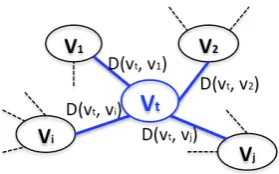
As previously mentioned, we decided to use the graph structure to characterize our dataset. In such a way, we take advantage of the graph’s properties, such as, the neigh-borhood, the edge weights, the size. We built a undirected graph for each term, each graph is independent from the others.
Graph construction: A graph (see Figure 2) for each biomedical term is built. Vertices denote terms, and edges denote co-occurrence relations between terms. Co-occurrences between terms are computed as the weight of the relation in the initial dataset. This relation is statistic-based by linking all co-occurring terms without considering their meaning or function in the text. Each graph is built with the first 1 000 terms extracted with BIOTEX applica-tion3 fromAt. The graph is undirected as the edges imply
that terms simply co-occur, without any further distinction regarding their role. We use theDice coefficient(calledD), a basic measure to compute the co-occurrence between two termsxandyin a text (i.e. title or abstract) in order to cre-ate the graph. Table 1 shows the 12 graph-based features.
Figure 2:Graph created for the termt.
In Figure 2,vtrepresents the vertex with the termt,vi
rep-resents a vertexiin the graph,N(vi)the neighborhood of
vi,|N(vi)|the number of neighbors ofvi,rj the neighbor
1) Number of Words:represented asnW ords(t), is the number of words that contains the termt. For instancenWords(Lung cancer)= 2.
2) Number of UMLS Terms:represented bytermsU(t), that is the number of UMLS terms contained in the set of abstractsAt.
3) Minimum of UMLS Terms:denoted asminU(t), represents the minimum number of UMLS terms contained for eachaofAt.
minU(t) =min(termsU(a1), termsU(a2), ...)
4) Maximum of UMLS Terms:denoted asmaxU(t), represents the maxi-mum number of UMLS terms contained for eachaofAt.
maxU(t) =max(termsU(a1), termsU(a2), ...)
5) Mean of UMLS terms: denoted asmeanU(t), represents the mean of number of UMLS terms for eachaofAt.
meanU(t) =1
n×
Pn
i=1termsU(ai)
6) Standard deviation of UMLS Terms:denoted assdU(t), represents the standard deviation of number of UMLS terms contained for eachaofA.
sdU(t) = 1
n−1×
pPn
i=1(termsU(ai)−meanU(t))2
7) Number of AGROVOC Terms: denoted astermsA(t), represents the number of AGROVOC terms contained in the set of abstractsAtoft. 8) Minimum of AGROVOC Terms:denoted asminA(t), is the minimum number of AGROVOC terms contained in eachaofAt.
minA(t) =min(termsA(a1), termsA(a2), ...)
9) Maximum of AGROVOC Terms:denoted asmaxA(t), is the maximum number of AGROVOC terms contained in eachaofAt.
maxA(t) =max(termsA(a1), termsA(a2), ...)
10) Mean of AGROVOC Terms:denoted asmeanA(t), represents the mean of number of AGROVOC terms for eachaofAt.
meanA(t) =1
n×
Pn
i=1termsA(ai)
11) Standard deviation of AGROVOC Terms:denoted assdA(t), represents the standard deviation of number of AGROVOC terms contained for eachaof
A. sdA(t) = 1
n−1×
pPn
i=1(termsA(ai)−meanA(t))2 Graph-based Features
1) Number of Neighbors:is the number of neighbors of vertexvtin the
in-duced graph. ng(v
t) =|N(vt)|
2) Sum of Edge Weights:denoted assum, represents the sum of edge weights specifically for the vertexvtin the graph created fort.
sum(vt) = ng(vt)
X
j=1
weight(vt, rj)
3) Minimum of Number of Neighbors:denoted asminNG, represents the minimum number of neighbors of allviin the graph created fort.
minN G(t) =min(ng(v1), ng(v2), ...)
4) Maximum of Number of Neighbors:denoted asmaxNG, represents the maximal number of neighbors of allviin the graph created fort.
maxN G(t) =max(ng(v1), ng(v2), ...)
5) Mean of Number of Neighbors:denoted asmeanNG, represents the mean of the number of neighbors of allviin the graph created fort.
meanN G(t) = P1000
i=1ng(vi) 1000
6) Standard deviation of Number of Neighbors:denoted assdNG, represents the standard deviation of the number of neighbors of allviin the graph created
fort.
sdN G(t) = √P1000
i=1(ng(vi)−meanN G(t))2
1000−1
7) Min of Sum of Edge Weights:denoted asminSUM, represents the mini-mum sum of edge weights of allvion the graph created fort.
minSU M(t) =min(sum(v1), sum(v2), ...)
8) Max of Sum of Edge Weights:denoted asmaxSUM, represents the maxi-mum sum of edge weights of allvion the graph created fort.
maxSU M(t) =max(sum(v1), sum(v2), ...)
9) Mean of Sum of Edge Weights:denoted asmeanSUM, represents the mean of sum of edge weights of allviin the graph created fort.
meanSU M(t) = P1000
i=1sum(vi) 1000
10) Standard deviation of Sum of Edge Weights:denoted assdSUM, repre-sents the standard deviation for the sum of edge weights of allviin the graph
created fort.
11) Number of Neighbors in UMLS:represented asngUMLS, is the number of terms being neighbors with the vertexvtin the graph and in turn are in
UMLS. ngU M LS(v
t) =|N(vt)|rj∈U M LS
12) Sum of Edge Weights in UMLS:assumUMLS, represents the sum of edge weights forvtthat are in UMLS for the graph created fort.
sumU M LS(vt) = ngU M LS(vt)
X
j=1
weight(vt, rj)
Example: An illustrative example on how to extract fea-tures has been submitted as supplementary material of this paper.
2.2.
Machine Learning Algorithm
We use some well-known supervised algorithms, imple-mented in the Weka4 software with the default parameters
per each algorithm, such as:
Naives Bayes (NB) Meta Bagging (MB) AdaBoost (AB) M5P Tree (M5P)
Tree Decision (TD) Multilayer Perceptron (NN) SVM (SVM) MultiClassClassifier Logistic (MCC)
2.3.
Extraction of New Features
We present new features based on statistical measures to characterize our dataset. They are extracted directly from the dataset and from an induced graph. We select appropri-ate learning algorithms to determine if a term is polysemic. The main idea, is to capture the characteristics of dataset from the structural shape and size of graph induced from the dataset. Totally 23 features are proposed, 11 direct and 12 from the induced graph. Their effectiveness are illustrated by comparing the results obtained by different supervised algorithms.
Notation: for each term t let At = ai the set of
ti-tles/abstracts of Medline containingt.
3.
Data and Results
3.1.
Gold Standard Dataset
Our dataset is composed of 406 ambiguous and not am-biguous entities. The amam-biguous entities have been ex-tracted from the MSH WSD5(Jimeno-Yepes et al., 2011) dataset, which consists of 106 ambiguous abbreviations, 88 ambiguous terms, and 9 which are a combination of both, for a total of 203 ambiguous entities. The rest of the dataset of 203 not ambiguous entities, built with the same method-ology from MSH WSD. This dataset is well-known in Word Sense Disambiguation literature applied to the biomedical domain. This dataset has been submitted accompanying this paper. Table 2 summarizes the details of our gold stan-dard dataset.
Description Dataset
Nb of Entities 406
Nb of Ambiguous Entities 203
Nb of Not Ambiguous Entities 203 Nb of Tokens of the Context of Ambiguous Entities 7 597 337 Nb of Tokens of the Context of Not Ambiguous Entities 8 294 378 Mean of Tokens for each Ambiguous Entity 37 425 Mean of Tokens for each Not Ambiguous Entities 40 859
Table 2:Details of our Gold Standard Dataset
3.2.
Results
In this section, we report experiments done to evaluate the performance of the new proposed features (in total twenty three). Algorithms cited in section 2.2. are evaluated with
4
http://www.cs.waikato.ac.nz/ml/weka/
5http://wsd.nlm.nih.gov/
a 10-cross-validation. Results are provided in terms of
Ac-curacy (A), Precision (P), Recall (R), andF-Measure (F)
over the dataset. In section 3.2.1., experiments are done with direct and graph-based features separately. We also wanted to explore the performance of the features by mix-ing the 11 direct features with the 12 graph-based features, these results are presented in section 3.2.2.. As major stud-ies deals with the identification of the correct meaning of a term, a comparison of our approach with others can not be provided. To our knowledge there are not studies focused in the detection of polysemy with binary output (i.e., true or false).
3.2.1. Direct and Graph-based Features
Table 3 shows the results obtained on our dataset with direct features (left side) and graph-based features (right side). We can see that M5 Model tree gets the best results with direct features, and Meta Bagging gets the best results with graph-based features. Both with anaccuracy(A) of 0.921. This means that the supervised algorithms with our direct features have classified correctly 92% instances (polysemic or not).
Direct Features Graph-based Features
A P R F A P R F
NB 0.860 0.863 0.860 0.859 0.860 0.863 0.860 0.859 AB 0.897 0.903 0.897 0.896 0.899 0.900 0.899 0.899 TD 0.879 0.882 0.879 0.879 0.882 0.884 0.882 0.882 SVM 0.919 0.922 0.919 0.919 0.874 0.875 0.874 0.874 MB 0.892 0.896 0.892 0.891 0.921 0.922 0.921 0.921
M5P 0.921 0.925 0.921 0.921 0.884 0.885 0.884 0.884 NN 0.906 0.907 0.921 0.906 0.906 0.907 0.906 0.906 MCC 0.914 0.915 0.914 0.914 0.914 0.914 0.914 0.914
Table 3:Direct and Graph-based Features
3.2.2. Combining two kinds of Features
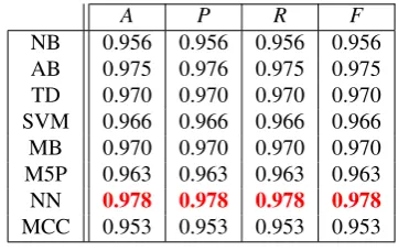
We study the effect of feature mixing, that means direct plus graph-based features. These two types of features are combined and Table 4 reports the results. We can see that Neural Network model (Multilayer Perceptron) gets excel-lent results, with anaccuracy(A) of 97.8%. This table il-lustrates as well that the minimal performance is 95.3% of accuracy. We can prove that the combination of two kinds of features gives the best results.
A P R F
NB 0.956 0.956 0.956 0.956
AB 0.975 0.976 0.975 0.975
TD 0.970 0.970 0.970 0.970
SVM 0.966 0.966 0.966 0.966
MB 0.970 0.970 0.970 0.970
M5P 0.963 0.963 0.963 0.963
NN 0.978 0.978 0.978 0.978
MCC 0.953 0.953 0.953 0.953
Table 4:Combining two kinds of Features
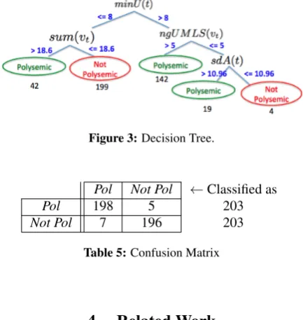
3.2.3. Discussion
tree (TD), in order to discuss the types of features high-lighting by this algorithm. Figure 3 shows the associated decision tree. We can see that only 4 of the 23 features have been taken into account for classification. Two di-rect (minU(t), sdA(t)) and two graph-based (sum(vt),
ngU M LS(vt)) features. The two direct features are
ex-tracted with UMLS (minU(t)) and AGROVOC (sdA(t)), this confirms that overlapping between the two dictionaries are useful to detect the biomedical term polysemy. We can observe in Figure 3 that the combination ofminU(t)and sum(vt)allows us to classify the mostnot polysemicterms,
199 of 203. Table 5 presents the confusion matrix, corre-sponding to an Accuracy (A) of 0.97 (see Table 4, column
A, rowTD).
Figure 3:Decision Tree.
Pol Not Pol ←Classified as
Pol 198 5 203
Not Pol 7 196 203
Table 5:Confusion Matrix
4.
Related Work
One related task to polysemy detection is the term am-biguity detection (TAD) (Baldwin et al., 2013), which given a term and a corresponding topic domain, determines whether the term uniquely references a member of that topic domain. For instance, given a term such as Brave
and a category such asfilm, the task is make a binary de-cision as to whether all instances ofBravereference a film by that name. In this case, the termBrave is already in-dexed in this category. In our case, we evaluate candidate terms that are not indexed. Another close study proposes a measure to decide if a preposition is polysemous to deter-mine the preposition senses (K¨oper and im Walde, 2014). In this case, the prepositions exist already in a terminol-ogy. This is similar to the well studied issues of named en-tity disambiguation (NED) and word sense disambiguation (WSD). These tasks assume that the number of senses of a word is given. This makes these tasks inapplicable in en-riching terminology tasks. One task that requires polysemy detection is word sense induction (WSI), which attempts to both figure out the number of senses of a word, and what they are. WSI uses unsupervised techniques to automati-cally identify the set of senses denoted by a word (Navigli, 2012; Wang et al., 2015). The main approaches to WSI proposed are categorized in four types: i)Context cluster-ing: The distributional profile of words implicitly expresses
their semantics, a well-known approach to context cluster-ing is the context-group discrimination algorithm (Sch¨utze, 1998; Van de Cruys and Apidianaki, 2011); ii)Word
clus-tering: Cluster words which are semantically similar and to
discover a sense, for instance the work of (Pantel and Lin, 2002); iii)Co-occurrence Graphs: These techniques have the same principle than the word clustering approaches, but they use graphs of word co-occurrences to identify the set of senses of a word (Navigli and Crisafulli, 2010), for in-stance some algorithms such as HyperLex (V´eronis, 2004), Pagerank (Agirre et al., 2006; Agirre and Soroa, 2009); and
iv) Probabilistic clustering: The objective is to formalize
WSI in a generative model. For each ambiguous word a distribution of senses is drawn (Lau et al., 2012; Brody and Lapata, 2009).
One area which extracts several kinds of features is Meta-learning. The objective is given a dataset to select a suit-able predictive model. The steps of Meta-Learning are: a) Meta-features extraction, and b) Evaluation and selection of the best learner algorithm to the dataset. Meta-features are categorized in 3 classes. The first one is based on sta-tistical and information-theoric characterization. The sec-ond one exploits properties of some induced hypothesis, for instance tree, graphs. The third one, landmarkers, uses in-formation obtained from the performance of learning algo-rithms as features. In this paper we investigated the two first types of meta-features in order to propose original tures (see Section 2.). The most frequent extracted fea-tures from datasets, are frequency, mean, standard devia-tion, etc. These measures have been used to extract meta-features according to an induced decision tree (Peng et al., 2002). The authors extracted 15 meta-features. Additional features have been proposed, as transformations of existing ones (Castiello et al., 2005), and some guidelines have been fixed to select the most informative ones. In their work, 9 new meta-features have been proposed. Other statistic meta-features have been presented in (Reif et al., 2012b), the authors added an additional feature selection method in order to automatically select the most useful measures. A similar work (Reif et al., 2012a) presented a new function, which is a novel data generator for creating datasets. As we saw, induced decision tree is in general used to extract features, but there is not approach based on graph models for feature extraction. Graphs are a very useful structure thanks to their properties.
5.
Conclusions and Perspectives
In this paper, we present a novel approach to predict if a term is polysemic focused on the biomedical domain. The main contribution of this paper is the definition of new fea-tures, which are directly extracted from the text dataset and from an induced graph. Our novel approach is based on the extraction of new features that characterize better our dataset. This allowed a more efficient classification task (polysemy prediction). For the classification we used the most well-known supervised algorithms over the whole fea-tures.
the best results. The results were calculated in terms of
Ac-curacy, Precision, RecallandF-Measure. We observed the
set of supervised algorithms on the features mixing got an accuracy (A) between 95.3% and 97.8%.
Next step is the use of the created graph, to determine the possible senses for poslysemic terms. Different perspec-tives can be considered in the future, such as increasing the number of features using other dictionaries like Wordnet associated to a general domain.
6.
Acknowledgements
This work was supported in part by the French National Re-search Agency under JCJC program, grant ANR-12-JS02-01001, as well as by University of Montpellier,CNRS, IBC of Montpellier project and the FINCyT program, Peru.
7.
Bibliographical References
Agirre, E. and Soroa, A. (2009). Personalizing pagerank for word sense disambiguation. In Proceedings of the 12th Conference of the European Chapter of the
Asso-ciation for Computational Linguistics, EACL ’09, pages
33–41. Association for Computational Linguistics. Agirre, E., Martinez, D., De Lacalle, O. L., and Soroa, A.
(2006). Evaluating and optimizing the parameters of an unsupervised graph-based wsd algorithm. In Proceed-ings of the first workshop on graph based methods for
natural language processing, pages 89–96. Association
for Computational Linguistics.
Agirre, E., L´opez de Lacalle, O., and Soroa, A. (2014). Random walks for knowledge-based word sense dis-ambiguation. Computational Linguistics, 40(1):57–84, March.
Baldwin, T., Li, Y., Alexe, B., and Stanoi, I. R. (2013). Automatic term ambiguity detection. InProceedings of the 51st Annual Meeting of the Association for
Compu-tational Linguistics, ACL ’13, pages 804–809,
Strouds-burg, PA, USA. Association for Computational Linguis-tics.
Brody, S. and Lapata, M. (2009). Bayesian word sense in-duction. InProceedings of the 12th Conference of the European Chapter of the Association for Computational
Linguistics, EACL ’09, pages 103–111. Association for
Computational Linguistics.
Castiello, C., Castellano, G., and Fanelli, A. M. (2005). Meta-data: Characterization of input features for meta-learning. In Modeling Decisions for Artificial
Intelli-gence, pages 457–468. Springer.
El-Rab, W. G., Zaiane, O. R., and El-Hajj, M. (2013). Biomedical text disambiguation using umls. In Proceed-ings of the 2013 IEEE/ACM International Conference on
Advances in Social Networks Analysis and Mining, pages
943–947. ACM.
Jimeno-Yepes, A. J., McInnes, B. T., and Aronson, A. R. (2011). Exploiting mesh indexing in medline to generate a data set for word sense disambiguation. BMC bioinfor-matics, 12(1):223.
K¨oper, M. and im Walde, S. S. (2014). A rank-based distance measure to detect polysemy and to determine salient vector-space features for german prepositions. In
Proceedings of the Ninth International Conference on
Language Resources and Evaluation (LREC’14), pages
4459–4466, Reykjavik, Iceland, May. European Lan-guage Resources Association (ELRA).
Lau, J. H., Cook, P., McCarthy, D., Newman, D., and Bald-win, T. (2012). Word sense induction for novel sense detection. InProceedings of the 13th Conference of the European Chapter of the Association for Computational
Linguistics, EACL ’12, pages 591–601. Association for
Computational Linguistics.
Navigli, R. and Crisafulli, G. (2010). Inducing word senses to improve web search result clustering. InProceedings of the 2010 conference on empirical methods in natural
language processing, EMNLP ’10, pages 116–126.
As-sociation for Computational Linguistics.
Navigli, R. (2012). A quick tour of word sense disam-biguation, induction and related approaches. In
SOF-SEM 2012: Theory and practice of computer science,
pages 115–129. Springer.
Pantel, P. and Lin, D. (2002). Discovering word senses from text. InProceedings of the Eighth ACM SIGKDD International Conference on Knowledge Discovery and
Data Mining, KDD ’02, pages 613–619, New York, NY,
USA. ACM.
Peng, Y., Flach, P. A., Soares, C., and Brazdil, P. (2002). Improved dataset characterisation for meta-learning. In
Discovery Science, pages 141–152. Springer.
Reif, M., Shafait, F., and Dengel, A. (2012a). Dataset gen-eration for meta-learning. 35th German Conference on Artificial Intelligence.
Reif, M., Shafait, F., and Dengel, A. (2012b). Meta2-features: Providing meta-learners more information.
35th German Conference on Artificial Intelligence.
Sch¨utze, H. (1998). Automatic word sense discrimination. volume 24, pages 97–123, Cambridge, MA, USA. MIT Press.
Van de Cruys, T. and Apidianaki, M. (2011). Latent se-mantic word sense induction and disambiguation. In
Proceedings of the 49th Annual Meeting of the Associ-ation for ComputAssoci-ational Linguistics: Human Language
Technologies-Volume 1, ACL ’11, pages 1476–1485,
Stroudsburg, PA, USA. Association for Computational Linguistics.
V´eronis, J. (2004). Hyperlex: lexical cartography for information retrieval. Computer Speech & Language, 18(3):223–252.
Wang, J., Bansal, M., Gimpel, K., Ziebart, B., and Yu, C. (2015). A sense-topic model for word sense induction with unsupervised data enrichment. Transactions of the
Association for Computational Linguistics, 3:59–71.
Zhong, Z. and Ng, H. T. (2012). Word sense disambigua-tion improves informadisambigua-tion retrieval. In Proceedings of the 50th Annual Meeting of the Association for
Compu-tational Linguistics, ACL ’12, pages 273–282,