Interferometers
Thesis by
Denis Martynov
In Partial Fulfillment of the Requirements for the Degree of
Doctor of Philosophy
California Institute of Technology Pasadena, California
2015
Acknowledgments
I am very grateful to my adviser Rana Adhikari for his support in most of my efforts and for his help to find my place in the field. Every day of my graduate schooling was different. I had an opportunity to work at the 40m prototype and LIGO Livingston Observatory as well as participate in various conferences and workshops. This experience and Rana’s advice helped me understand how to be part of a big team and contribute to commissioning of LIGO interferometers.
I would like to thank Valera Frolov for his support during our commissioning work at LIGO Livingston Observatory. His deep understanding of the instrument and strong common sense guided our team towards robust lock acquisition and fruitful noise hunting at the Livingston site. Valera helped me, as well as many other students at the site, to believe that we can become successful scientists.
Many thanks to Peter Fritschel, Matt Evans, Lisa Barsotti, Rainer Weiss, and Nergis Mavalvala for many interesting ISC meetings, discussions of current and future LIGO research, and for their support and interest in my work at LIGO.
I would like to thank LIGO Caltech staff and in particular 40m team. I appreciate all the help from Koji Arai, Steve Vass, Aidan Brooks, Jan Harms, Alan Weinstein, Hiro Yamamoto, Gabriele Vajente, Nicolas Smith, Suresh Doravari, Jameson Rollins, Eric Gustafson, and Jenne Driggers.
It was a pleasure for me to work with Livingston local staff, students, operators, installation, detector characterization, and calibration groups. I am thankful for their help, networking and frequent discussions about the instrument. In particular, I would like to thank Adam Mullavey, Shivaraj Kandhasamy, Stuart Aston, Zach Korth, Jan Poeld, Anamaria Effler, Ryan DeRosa, Arnaud Pele, Gary Traylor, Tom Evans, Richard Oram, Brian O’Reily, Joseph Betzwieser, Goe Giaime, Janeen Romie, and Melanie McCandless.
Abstract
Laser interferometer gravitational wave observatory (LIGO) consists of two complex large-scale laser interferometers designed for direct detection of gravitational waves from distant astrophysical sources in the frequency range 10Hz - 5kHz. Direct detection of space-time ripples will support Einstein’s general theory of relativity and provide invaluable information and new insight into physics of the Universe.
The initial phase of LIGO started in 2002, and since then data was collected during the six science runs. Instrument sensitivity improved from run to run due to the effort of commissioning team. Initial LIGO has reached designed sensitivity during the last science run, which ended in October 2010.
In parallel with commissioning and data analysis with the initial detector, LIGO group worked on research and development of the next generation of detectors. Major instrument upgrade from initial to advanced LIGO started in 2010 and lasted until 2014.
This thesis describes results of commissioning work done at the LIGO Livingston site from 2013 until 2015 in parallel with and after the installation of the instrument. This thesis also discusses new techniques and tools developed at the 40m prototype including adaptive filtering, estimation of quantization noise in digital filters and design of isolation kits for ground seismometers.
The first part of this thesis is devoted to the description of methods for bringing the inter-ferometer into linear regime when collection of data becomes possible. States of longitudinal and angular controls of interferometer degrees of freedom during lock acquisition process and in low noise configuration are discussed in details.
Once interferometer is locked and transitioned to low noise regime, instrument produces astro-physics data that should be calibrated to units of meters or strain. The second part of this thesis describes online calibration technique set up in both observatories to monitor the quality of the collected data in real time. Sensitivity analysis was done to understand and eliminate noise sources of the instrument.
are described in the last part of this thesis. Applications of optimal time domain feedback control techniques and estimators to aLIGO control loops are also discussed.
Contents
Acknowledgments iii
Abstract iv
1 Introduction 1
1.1 Gravitational waves . . . 2
1.2 Source of gravitational waves . . . 3
1.2.1 Bursts . . . 4
1.2.2 Continuous waves . . . 4
1.2.3 Binary systems . . . 5
1.2.4 Stochastic background . . . 5
1.3 Measurement technique . . . 5
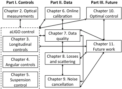
1.4 Structure of this thesis . . . 7
2 Optical detection scheme 9 2.1 Optical measurements . . . 9
2.1.1 Length stabilization . . . 10
2.1.1.1 Homodyne detection. . . 11
2.1.1.2 Heterodyne detection . . . 13
2.1.1.3 Length dithering . . . 15
2.1.1.4 Phase locking. . . 16
2.1.2 Angular stabilization. . . 17
2.1.2.1 DC sensing . . . 18
2.1.2.2 RF sensing . . . 19
2.1.2.3 Angle dithering . . . 21
2.1.3 Mode matching . . . 21
2.2 aLIGO optical design. . . 22
2.2.1 Michelson interferometer. . . 23
2.2.3 Dual recycled Michelson interferometer . . . 28
2.2.4 Dual recycled Fabry Perot Michelson interferometer . . . 29
3 Lock acquisition and longitudinal control 31 3.1 Arm length stabilization . . . 32
3.2 DRMI locking. . . 35
3.3 CARM offset reduction . . . 38
3.3.1 CARM control . . . 39
3.3.2 DARM control . . . 41
3.4 DC readout . . . 42
4 Alignment and angular motion stabilization 45 4.1 Interferometer initial alignment . . . 46
4.1.1 Alignment sequence . . . 46
4.1.2 Alignment precision . . . 48
4.2 DRMI angular motion . . . 49
4.2.1 ABCDEF model of power recycling cavity . . . 49
4.2.2 Angular controls . . . 52
4.3 Angular controls during CARM offset reduction. . . 53
4.4 Angular motion stabilization in full lock . . . 55
5 Suspension control 58 5.1 Longitudinal control . . . 59
5.1.1 ALS DIFF loop. . . 59
5.1.2 DARM control using L2 stage. . . 62
5.1.3 L2/L3 crossover . . . 64
5.2 Damping of high-Q modes . . . 67
5.2.1 BS bounce and roll damping . . . 68
5.2.2 Quad bounce and roll damping . . . 70
5.2.3 Quad violin mode damping . . . 71
6 Instrument calibration 74 6.1 Front end model . . . 74
6.2 Actuator calibration . . . 76
6.2.1 Michelson interferometer. . . 76
6.2.2 ALS beat notes . . . 78
6.2.3 Photon calibrator. . . 79
6.4 Total DARM calibration . . . 81
7 Data quality 83 7.1 Fundamental noises. . . 85
7.1.1 Quantum noise . . . 85
7.1.2 Thermal noise . . . 87
7.1.3 Seismic noise . . . 88
7.2 Charging noise . . . 91
7.3 Sensing and actuation . . . 95
7.3.1 Electrostatic driver. . . 95
7.3.2 Penultimate mass actuators . . . 96
7.3.3 Local damping . . . 96
7.3.4 OMC electronics . . . 96
7.4 Auxiliary loops . . . 97
7.4.1 Angular controls . . . 97
7.4.2 Laser frequency noise . . . 99
7.4.3 DRMI noise . . . 99
7.5 Intensity and jitter . . . 101
7.5.1 Input amplitude noise . . . 101
7.5.2 Input beam jitter noise . . . 103
7.6 Residual gas. . . 104
7.7 Lines . . . 105
7.8 Parametric instability . . . 106
7.9 Glitches . . . 107
7.9.1 DAC zero crossings. . . 107
7.9.2 Frequency and intensity transients . . . 108
7.9.3 Data transmission errors. . . 109
7.9.4 OMC backscattering . . . 109
7.9.5 Optical levers . . . 109
7.10 Discussion . . . 109
8 Losses and scattering 111 8.1 Arm losses. . . 111
8.2 Output losses . . . 114
8.3 Noise from scattered light . . . 115
8.3.1 Interferometer input . . . 117
8.3.3 In-air paths and chamber walls . . . 118
8.3.4 Output mode cleaner. . . 121
8.4 Mitigation techniques . . . 122
8.4.1 Feedforward cancellation. . . 123
9 Feedforward noise cancellation 126 9.1 Auxiliary length loops . . . 127
9.2 Angular controls . . . 131
9.3 Seismic noise . . . 132
9.3.1 Static filter . . . 133
9.3.2 Adaptive filters . . . 135
10 Optimal feedback control 140 10.1 Linear quadratic regulator . . . 141
10.1.1 State-space augmentation . . . 141
10.1.2 Applications to LIGO . . . 142
10.2 Kalman filter . . . 143
10.2.1 Test mass curvature estimation . . . 145
10.3 H∞ control technique . . . 148
10.3.1 Optical lever damping . . . 150
10.3.2 Local damping . . . 151
10.4 µ-synthesis . . . 153
10.4.1 Robust local damping . . . 154
11 Future work 156 11.1 Short term upgrades . . . 157
11.2 Medium term improvements . . . 159
11.2.1 Interferometer control . . . 159
11.2.2 OMC backscattering . . . 160
11.2.3 Data analysis and detector performance . . . 161
11.3 Variable finesse of the signal recycling cavity . . . 163
Summary and conclusions 167 A Acronyms 169 B Quantization noise 171 B.1 Estimation algorithm. . . 173
C Suspension wire heating 175
D Beam clipping in Michelson interferometer 177
E Seismometer isolation kit 181
List of Figures
1.1 Effect of gravitational wave on Michelson interferometer. . . 6
1.2 Structure of this thesis. . . 7
2.1 S-polarized laser beam incident on moving interferometer mirror. . . 10
2.2 Homodyne detection scheme and error signals in Michelson and Fabry-Perot interfer-ometers.. . . 12
2.3 Heterodyne detection scheme and error signals in Michelson and Fabry-Perot interfer-ometers.. . . 15
2.4 Locking Fabry-Perot cavity using auxiliary laser. . . 17
2.5 Cavity, input, and central axes of a misaligned Fabry-Perot cavity. . . 18
2.6 Sensing of Fabry-Perot cavity axis motion using two QPDs in transmission. . . 18
2.7 Fabry-Perot cavity alignment scheme using RF sensors. . . 20
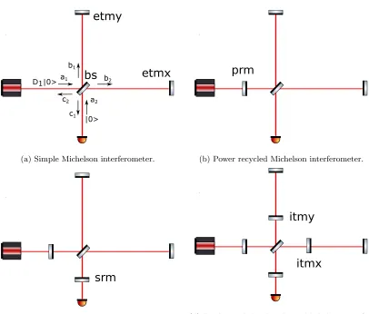
2.8 Optical configurations for gravitational wave detection. . . 24
2.9 Quantum noise coupling to gravitational wave channel in different optical configurations when interferometer input power is 125W.. . . 28
3.1 Stabilization of arm cavities using auxiliary lasers. . . 33
3.2 Measured ALS COMM noise. Blue trace shows ALS COMM noise measured when X-arm was controlled using PDH signals. Orange trace shows residual longitudinal noise measured by PDH signals when low passed ALS COMM signal is used for IMC length control. . . 34
3.3 DRMI control using REFL PDH signals. . . 35
3.4 Response of REFL heterodyne signals to PRCL, MICH, and SRCL detuning. . . 36
3.5 Signals used to control interferometer during CARM offset reduction. . . 38
3.6 TRX and REFL9I signals depending on CARM offset. . . 40
3.8 DARM transition from ALS DIFF to AS45Q/√T RX is done when CARM offset is
100pm. A slow servo corrects DARM DC offset when CARM offset is between 250pm
and 100pm. . . 41
3.9 Signals used to control interferometer in full lock. . . 42
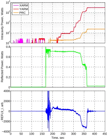
3.10 Interferometric signals during the process of lock acquisition. Input power of interfer-ometer is 0.75W. . . 43
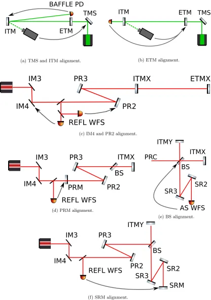
4.1 Steps of interferometer initial alignment. First, arm cavities are aligned using green beam and serve as a reference to power and signal recycling cavity axis, BS and input beam. . . 47
4.2 Seismically driven angular motion of input mirrors (IM), small triple suspensions (HSTS), large triple suspensions (HLTS), beam splitter suspension (BSFM) and quadru-ple suspensions (QUAD). . . 49
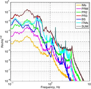
4.3 Linear coupling of seismic motion to PRC power fluctuations.. . . 51
4.4 Response of AS A and B WFS to DHARD mode during CARM offset reduction. . . . 54
4.5 Angular controls of the full interferometer. . . 56
4.6 Optical power resonating in the power recycling cavity during 30 hour lock stretch. Interferometer input power is 22 Watts. . . 57
5.1 Open loop transfer function of ALS DIFF loop and M0, L1 and L3 stages. Loop is unconditionally stable when it is being engaged and M0 gain is lower than nominal. Then boost is turned on to suppress low frequency motion and M0 gain is increased. . 60
5.2 ALS DIFF loop suppression and control signal to L1 and L3 stages. . . 61
5.3 Compensation filter from quad L2 to L3 stage. . . 62
5.4 Control signal to L2 stage. . . 63
5.5 Wide violin resonance.. . . 64
5.6 Bringing L2/L3 crossover in full lock. . . 65
5.7 DARM control scheme. Prepresents transfer functions from L3, L2, L1, and M0 stages to DARM,C - correction filters,G0 - DARM control servo,G- crossover filters. . . . 66
5.8 Control signal to L2 and L3 stages using L2/L3 crossover. . . 67
5.9 Phase sectors of open loop transfer functionH. . . 68
5.10 Open loops transfer function of BS bounce mode damping. . . 69
5.11 Comparison of BS longitudinal transfer function. . . 70
5.12 Excitation and damping of ITMX violin modes. Top plot shows control signal to suspension L2 actuator. Bottom plot shows amplitude of violin mode. . . 73
6.2 Beam splitter calibration using Michelson interferometer. . . 77
6.3 Calibration of L2 stage actuator using ALS DIFF beatnote. . . 78
6.4 Measurement of the DARM pole.. . . 80
6.5 Comparison of DARM open loop transfer functions obtained from the calibration model and loop sweep. . . 81
6.6 Check of the final DARM calibration using photon calibrators. . . 82
7.1 Interferometer optical configuration in low noise regime. . . 84
7.2 DARM sensitivity curve and known noise couplings. . . 85
7.3 Coupling of fundamental noises to DARM. . . 86
7.4 Seismic noise and motion of isolated optical tables during summer and winter time. . 89
7.5 Transfer function from longitudinal table motion to optic motion. . . 90
7.6 Side view of ETM with electrostatic blades, lower and upper ring heaters and metal cage.. . . 91
7.7 Transfer function from electrostatic blades and TCS ring heater to DARM. . . 92
7.8 Potential noise coupling to DARM through static charge on end test masses. . . 94
7.9 Sensing and actuation noise coupling to DARM. . . 95
7.10 Coupling from auxiliary length and angular loops to DARM. . . 97
7.11 Angular motion of test masses in pitch degree of freedom measured by AS45Q WFS.. 98
7.12 Angular motion of test masses in yaw degree of freedom measured by AS45Q WFS. . 98
7.13 MICH noise budget. . . 100
7.14 SRCL noise budget. . . 100
7.15 PRCL noise budget. . . 101
7.16 Coupling of laser amplitude noise and beam jitter to DARM. Orange trace shows DARM spectrum with broken PZT of PMC which created high frequency intensity and jitter noise. . . 102
7.17 Input RIN coupling to OMC RIN. . . 103
7.18 Coupling of squeezed film damping and noise from residual gas in the arms to DARM. 104 7.19 Excitation and ringing down of the test mass body mode due to parametric instability. 106 7.20 Glitches in PRCL error signal due to PRM M3 DAC zero crossing. . . 107
7.21 Glitches in frequency and intensity servos depending on IMC VCO control signal cali-brated to kHz. . . 108
7.22 Improvements in DARM sensitivity from June 2014 up to March 2015. . . 110
8.1 Dependence of power recycling gain and interferometer visibility on intracavity losses. 112 8.2 Round trip loss measurement depending on beam position on ITM. . . 113
8.4 Dependence of optical losses in X- and Y-arm on different beam offsets from the optic
center.. . . 114 8.5 Simulation and measurement of OMC transmitted power in dependence of DARM offset.115
8.6 Backscattering from moving objects. Light backscatters from intracavity baffles or
chamber walls, output Faraday isolator and mode cleaner. . . 116 8.7 Range fluctuations due to alignment drift.. . . 116 8.8 Scattered light noise at the interferometer input degrades behavior of intensity
stabi-lization servo.. . . 117 8.9 Comparisons of seismic noise with motion of X- and Y-arm tubes. If tube is insulated
then motion in directions perpendicular to the cavity axis is significantly reduced above
20Hz. . . 118 8.10 Scattered light noises from in-air beams.. . . 119 8.11 Scattering from the output port. Orange trace shows scattering shelves seen in DARM
if motion of HAM5 ISI is increased by 1um/sec. Pink trace shows scattered light noise
if HAM6 fans are turned on. Fans increase acoustic noise around HAM6 chamber by
factor of 3 around 70Hz and factor of 10 at higher frequencies. . . 120 8.12 Measurement of output port reflectivity. . . 122 8.13 Simulation of scattering noise coupling to DARM. Scattering shelf comes from large
low freqency motion. Coherence between DARM and high frequency motion of the
scattering object depends on low frequency motion. . . 124 8.14 Coherence between accelerometers installed on the same wall on HAM6 chamber. . . 125
9.1 Simplified scheme of feedforward subtraction. Noise source couples to gravitational
wave channel with transfer functionT. Noise is measured by witness instrument with
transfer functionS, and is conditioned and canceled from DARM using actuatorA. . 127 9.2 Coherence between DARM and auxiliary length degrees of freedom. Red trace shows
coherence with MICH. Blue trace shows coherence with SRCL. . . 128 9.3 Simulated and measured MICH and SRCL coupling to DARM. . . 129 9.4 Online feedforward subtraction scheme of MICH and SRCL from DARM. . . 130 9.5 DARM spectrum with and without online feedforward subtraction of MICH and SRCL. 130
9.6 Online feedforward subtraction scheme of angular controls noise. Noise couple through
beam offcentering or coil imbalance x and is subtracted with feedforward filter K.
Transfer functions AP2P and AL2L denote actuator transfer function for angle and
length actuation. . . 131 9.7 Fitting of FIR filter with 10000 coefficients using IIR filter with 10 poles and zeros
9.8 Result of static feedforward subtraction using static Wiener filtering technique. Red
trace shows initial target signal before subtraction. Green curve is residual signal after
applying FIR Wiener filter. Blue trace shows residual motion after applying IIR filter
obtained by fitting optimal FIR filter. Black trace shows residual motion after installing
IIR filter in the online system. . . 135 9.9 Test of LMS adaptive filters at the 40m prototype. Seismometers are located in the
corner and end stations. . . 136 9.10 Online adaptive seismic noise cancellation scheme using FxLMS algorithm. . . 137 9.11 Norm of the filter coefficient vector during convergence process of FxLMS filter. . . . 138 9.12 Feedforward subtraction of seismic noise from IMC and arms.. . . 139
10.1 Application of LQR technique to BS optical lever servo. . . 143 10.2 Test mass and ring heater. . . 146 10.3 Norm of Kalman gain during the process of iterative solution of equations 10.13. . . . 147 10.4 Estimation of test mass radius of curvature using model and measurement. . . 148 10.5 Application ofH∞ technique to LIGO suspension control problems. . . 149
10.6 Application ofH∞ technique to BS optical lever damping. Blue trace shows BS pitch
to pitch transfer function when loop is open, and orange trace shows the same transfer
function when loop is closed. . . 150 10.7 Magnitude of control cost functions developed for design ofH∞controllers. . . 151
10.8 Simulation of damping BS suspension modes usingH∞controller. . . 152
10.9 Transfer function of BS top stage in longitudinal degree of freedom. Black trace
corre-sponds to the case when BS is undamped, red trace - damped usingH− ∞controller. 153
10.10 Frequency shape of position and control cost function generated for longitudinal
damp-ing of BS suspension. . . 154 10.11 Damping of BS longitudinal resonances using robust controller. . . 155 10.12 BS longitudinal displacement due to sensor noise. . . 155
11.1 Interferometer quantum noise depending SRM transmissionT and detuning of signal
recycling cavitya. . . 162 11.2 Compound SR2 mirror inside the signal recycling cavity.. . . 163 11.3 Power transmission and reflection phase from compound SR2 mirror based on cavity
detuning. . . 164 11.4 Interferometer quantum noise with SR2 cavity depending on cavity detuning and mass
of the mirrors. . . 165 11.5 Comparison of SRCL quantum noise in aLIGO configuration and with compound SR2
B.1 Filter forms used in initial and advanced LIGO to compute output of SOS. . . 172
B.2 DARM filter bank. Algorithm downloads input signal and computes output using two types of variables to estimate quantization noise of digital filters that are engaged. . . 173
B.3 Quantization noise of HAM ISI vertical damping loop. Noise is lower if ”biquad” form is used instead of direct form 2.. . . 174
C.1 Drift of BS pitch after lock is lost. Blue trace shows intracavity power measured by POP18 signal, red - BS pitch, magenta - BS yaw angle measured by optical lever. POP18 signal is negative when PRC is locked on carrier. This signal goes to zero when lock is lost. When PRC was locked, intracavity power was 60W. . . 176
C.2 Frequency shift of PR3 violin modes when input power was increased from 3W up to 10W. This shift confirmed that wires are heated by optical power resonating in the power recycling cavity.. . . 176
D.1 Power recycling gain, Michelson contrast defect and ring heater power during TCS test. Power on ring heaters was increased in steps to monitor effects in recycling gain and contrast defect. . . 178
D.2 Measurement of PRC g-factor during TCS test.. . . 179
D.3 Power recycling gain, Michelson contrast defect and cavity visibility during CO2 laser test. Power of CO2 beam power was slowly increased from 0 up to 175mW. . . 180
E.1 Assembly of the seismometer isolation kit.. . . 182
E.2 Guralp seismometer installed in the seismic isolation kit with internal cabling. . . 182
E.3 Drawing of granite block. . . 183
E.4 Drawing of connector plate for Guralp seismometer kit. . . 184
List of Tables
3.1 PRMI lock statistics.. . . 37
3.2 DRMI lock statistics. . . 37
3.3 Signals used for DRMI control during CARM offset reduction. Correction gain α is tuned to subtract PRCL from SRCL error point. . . 37
3.4 Signals used for CARM control. . . 39
3.5 Signals used for DARM control. . . 41
4.1 Table shows PRC waist position and tilt motion as well as power build up in the cavity relative to maximum value when each specified optic is misaligned by 1 urad. Last four columns show beam spot shift on each optic. . . 51
4.2 Simulation of WFS response to angular motion of the mirrors during CARM offset reduction. Interferometer input power was set to 1W, and sensors get all optical power from interferometer. . . 53
4.3 Sensing matrix of angular sensors to test masses, IM4 and PR2 in full lock. Input PSL power during the measurement was 2W. Sensing matrix scales linearly with power up to 25W. . . 55
5.1 Possible outcomes of tuning procedure of the servo phase. Initial sector indicates servo phase from figure 5.9 when onlyBPf0 is used. . . 68
5.2 Test mass bounce and roll damping parameters. . . 71
5.3 Test mass violin modes damping parameters. . . 72
5.4 Damping parameters of second harmonics of test mass violin modes. . . 72
7.1 Measured projections of electrostatic forces due to charge on test masses and surround-ing metal on longitudinal direction. . . 93
8.1 Optical loss from individual components. . . 115
8.2 Scattered light noise from arm cavities. . . 118
Chapter 1
Introduction
Einstein’s theory of general relativity [1] extends Newton’s laws of universal gravitation towards large velocities and big gravitational potentials of interacting objects. General relativity could explain and predict many important physical effects including precession of the perihelion of the orbits of planets, angular deflection of light rays by gravity and gravitational lensing, frequency shift of light, and gravitational time dilation, existence of black holes, and other compact objects and radiation of gravitational waves.
The general theory of relativity provides a description of gravity as a geometric property of space and time. The presence of energy and momentum changes the curvature of space-time according to Einstein equations. Gravitational waves are ripples of space-time curvature that propagate outward from the source. Energy loss of a binary star system due to gravitational radiation was indirectly observed by Hulse and Taylor [2].
The mission of LIGO is to directly detect gravitational waves of cosmic origin and extract infor-mation about the source from the wave properties [3, 4]. This discovery will build a new branch of astronomy that will complement electromagnetic telescopes and neutrino observatories.
Advanced LIGO [5] is designed for broadband detection of gravitational waves in the frequency range from 10Hz up to 5kHz. US hosts two interferometers located at Livingston, LA and Hanford, WA. Using data from two sites, it is possible to correlate the gravitational wave signal and reduce the probability of false detection due to instrument glitches and noises. The Livingston and Hanford observatories are located 2998km apart and it takes 10msec for light to travel the distance between the two sites. Separation between the two observatories allows one to estimate the direction in the sky of the gravitational wave source.
Two other interferometers outside of U.S. are now under construction with design and sensitivity similar to aLIGO. The first one is the Italian-French VIRGO [6] instrument located in Pisa, and the second one is the Japanesse project KAGRA [7] located in the Kamioka mine. Yet another element of the worldwide network of gravitational wave detectors is proposed to be built in India [8].
interferometers [11], and torsion bar antennas [12]. These techniques can be used as low frequency gravitational wave detectors and complement large-scale optical interferometers.
Ground motion and available space for building instruments are the most significant challenges in detecting gravitational waves below 1Hz using terrestrial based instruments. For this reason space based detectors such as LISA [13] and DECIGO [14] were proposed in the past and research studies are currently undergoing.
This chapter gives an introduction to the concept of gravitational waves and astrophysical sources. The first section describes treatment of gravitational waves as small ripples in space time. The second section describes types of astrophysical sources of gravitational waves. The third section shows response of the Michelson interferometer to gravitational wave signal.
1.1
Gravitational waves
Since all objects move in gravitational fields in the same way independent of the object mass, the equivalence principle states that it is possible to cancel gravitational forces locally by moving to non-inertial reference frame. In this frame intervaldsis determined by the quadratic form
ds2=gijdxidxj (1.1)
wheregij is a metric tensor andxi are coordinates in four dimensional space-time.
In the absence of gravitational field, metric gij =ηij ≡diag(1,−1,−1,−1) in the inertial
ref-erence frame if Cartesian coordinates are used. Space-time is flat in this case. In the presence of gravitational field metricgij can not be brought to diagonal form by any coordinate transformation.
In this case space-time is curved.
If space-time metric tensor gij is known, motion of the object is determined by its geodesics
equation [15]:
Metric tensorgijdepends on matter and energy distribution and is determined by Einstein
equa-tions. These equations are nonlinear partial differential equations due to the fact that gravitational fields carry energy and momentum themselves. This is in contrast with linear Maxwell’s equations since electromagnetic field does not carry charge. Einstein equations can be written as [16]:
whereTikis the energy-momentum tensor,Rik= (
andGis the gravitational constant.
Einstein equations for space-time metricgij are usually solved numerically. Precise solutions are
known for limited cases of matter and energy distributions. Kerr metric [17] is a solution for empty space-time around a rotating uncharged axially-symmetric black hole with a spherical event horizon. Schwarzschild metric [18] describes gravitational field outside a spherical mass, on the assumption that the electric charge of the mass, angular momentum of the mass and universal cosmological constant are all zero. Reissner-Nordstrom metric [19] is a static solution which corresponds to the gravitational field of a charged, non-rotating, spherically symmetric body of mass M. KerrNewman metric [20] describes the space-time geometry in the region surrounding a charged, rotating mass.
In the weak field approximation far away from the source space-time metric is close to the diagonal formηij=diag(1,−1,−1,−1):
gij=ηij+hij (1.4)
where hij 1 is a small perturbation. Using gauge invariance, and up to first order in h, it is
possible to write Ricci tensor asRik= 12(52−c12
∂2
∂t2)hik. Einstein equations in the empty space are
reduced to:
Thus, elements of hij represent a plane wave propagating with the speed of light c. In the
transverse traceless gaugehij is given in the form [21]:
hij =
whereh+andh×represent two orthogonal polarizations of the gravitational wave with frequency
ω and wave vectork.
1.2
Source of gravitational waves
quadruple momentI. Retarded potential solution of Einstein equations can be written as [22]:
hij(t) =
2G
rc4I¨ij(t−R/c) (1.7)
LIGO studies all possible types of sources of gravitational waves that can be detected on Earth. However, since there are ambiguities in the models of gravitational radiation, all estimations of detection rates are considered to be approximate with a precision of one, two or even three orders of magnitude.
1.2.1
Bursts
Both electromagnetic and neutrino detectors periodically see short transient signals coming from the sky. Fast catastrophic processes in the Universe should also produce gravitational waves. In the general case, waveform of such events cannot be foreseen. Detection primarily relies on a coincidence of excess power in multiple detectors and synchronizing signal arriving time with electromagnetic and neutrino observatories.
Supernovae are potential sources of gravitational waves [23]. An explosion may be triggered by the re-ignition of nuclear fusion in a degenerate star or the gravitational collapse of a massive star. In the latter case of supernova explosion energy is released in the form of neutrinos, photons and also the gravitational waves.
Gamma ray bursts are associated with distant energetic explosions and can be also accompanied by gravitation wave emission [24]. This and other unforeseen astrophysical events have the potential of revealing new discoveries [25]
1.2.2
Continuous waves
Continuous waves are produced by the systems with asymmetry which rotate with constant and well-defined frequency [26]. Searching for these signals is a computationally demanding task due to the frequency modulation produced by Earth motion around the Sun. @EinsteinHome program [27] was started to use spare computational time on computers of registered volunteers.
1.2.3
Binary systems
Two compact objects orbiting around their common center of mass lose energy in the form of gravitational waves [29]. Energy loss makes objects gradually approach each other, and frequency of the orbit increases. At the end-of-life stage gravitational waves from the binary system can be detected in the frequency range of the ground based detectors 10Hz−5kHz.
Binary systems can consist of two neutron stars, two black holes, or a neutron star and a black hole. Waveforms coming from the merger of black holes are well modeled based on the general theory of relativity [30]. Merger of binary neutron stars is less understood due to tidal effects.
1.2.4
Stochastic background
The stochastic signal has an approximately constant amplitude and a broad continuous spectrum. These signals are not periodic and not impulsive. Stochastic background can be detected by cross correlating data from two or more detectors [31,32].
Cosmic gravitational wave background can arise from a large number of random events that oc-curred after the Big Bang. In this case waves are stretched as the Universe expands, and information about the early universe can be extracted after detection.
One more interesting source is the superposition of the signals from the vast population of compact binaries. Frequencies of emitted gravitational waves lie in the range from 1Hz up to several kHz depending on the mass distribution and time of formation [33].
1.3
Measurement technique
Fluctuations of strain are rather small, and significant effort is required to detect gravitational waves. Current section shows that Michelson interferometers can be used as gravitational wave detectors with high sensitivity. In this optical configuration light from the laser is split on the beam splitter, and travels along perpendicular arms to the end mirrors, bounces back, and recombines on the beam splitter. Figure1.1 shows the effects on the Michelson interferometer when a gravitational wave of + polarization is incident from the top on the setup.
Disturbance of relative arm length produces a signal to the antisymmetric port of the Michelson interferometer. Differential phase shift due to gravitational wave in + polarization can be computed from geodesic equation for light. Time dt required for the light to travel distancedl along X-arm can be written as:
ds2= (ηij+hij)dxidxj=dt2−(1 +h+)dl2= 0
dt=p1 +h+dl
Similarly, time required for the light to travel distancedlalong Y-arm isdt=p
1−h+dl. Total phase difference between X- and Y-arm beams after their reunion on the beam splitter is
4ϕ=ϕx−ϕy =
2πc
λ (τx−τy) =
4π λ (
Z L
0
p
1 +h+dl−
Z L
0
p
1−h+dl) (1.9) Since space-time metric perturbation h+<<1, it is possible to write:
4ϕ≈4π
λ
Z L
0
h+dl (1.10)
If the length of each interferometer arm is much smaller than gravitational wavelengthLλGW,
the instrument will detect arm length shift proportional to perturbation of space-time metric:
4L=h+L (1.11)
Two arms of Michelson interferometer are tuned to have equal macroscopic length L to reject laser frequency noise at the antisymmetric port. Gravitational waves in the×polarization produce phase shifts common to the interferometer arms and do not produce a signal at the antisymmetric port.
Figure 1.1: Effect of gravitational wave on Michelson interferometer.
Optical configuration of interferometer is optimized for the best sensitivity to gravitational waves in the frequency range 10Hz - 5kHz. For this purpose auxiliary degrees of freedom are introduced in LIGO interferometers, such as arm cavities and power, and signal recycling cavities. Chapter
1.4
Structure of this thesis
The first part of this thesis describes lock acquisition, alignment and control of advanced LIGO detectors. Chapter 3 and 4 are devoted to the sensing side of control loops and significantly rely on chapter2 with summarizes interferometric measurement and optical design of advanced LIGO. Chapter5 is devoted to actuation side of control loops and describes control of multi-stage suspen-sions and damping of high-Q modes.
The second part of this thesis is devoted to data quality and sensitivity of the instrument. Chapter 6 describes online calibration of advanced LIGO interferometers. Chapter 7 is devoted to broadband sensitivity analysis of the instrument data, narrow band lines and glitches found in data. Chapter8 describes measurement of optical losses in the arm cavities and noises coming from scattered light. Chapter9describes feedforward noise cancellation techniques to reduce coupling of auxiliary loops and seismic noise to gravitational wave channel.
The third part of this thesis describes ideas for future research. Chapter10is devoted to simula-tions and online tests of optimal feedback control loops and state estimation techniques. Chapter11
describes possible future improvements to advanced LIGO optical and mechanical configurations.
Chapter 2. Op,cal
Angular controls
Chapter 5.
Chapter 2
Optical detection scheme
This chapter describes how lasers, optical interferometers, and photodetectors can be used as strain meters. The problem of gravitational wave detection is reformulated to the problem of distance measurement between suspended test masses. Stabilized lasers are widely used for precision exper-iments, and a variety of commercial optical components are available on the market, such as high quality mirrors, low-noise photodetectors, and stable lasers.
The first section of this chapter describes how lasers can be used for precision measurements. Pound-Drever-Hall [34] and DC readout techniques are currently used to control aLIGO optical cavities. In both cases readout signal is achieved by non-linear mixing of phase modulated light coming out from the interferometer with the light of a reference frequency. Optical power measured on the photodetector contains information about motion of interferometer mirrors relative to the laser wavelength.
The second section describes aLIGO optical configuration. Four test masses form two arm resonators, and the gravitational wave signal is derived from the differential length of these two arms. Common arm length is used to stabilize the laser. Beam splitter is used to equally split input laser beam between the arm cavities. The simple Michelson interferometer formed by the beam splitter and input test masses is controlled to keep the interferometer antisymmetric port at dark fringe. Power and signal recycling cavities installed at the input and output ports of interferometer are used to optimize sensing noise in the frequency range 10Hz - 10kHz.
2.1
Optical measurements
Longitudinal and angular motion of the mirrors can be measured using properties of light. Test mass is a part of the interferometer, and its motion is measured relative to other mirrors rather than to inertial frame. This limitation is not important for aLIGO since the gravitational wave signal is derived from the distance between test masses.
pro-duces a coherent optical wave of known frequency and spatial mode. aLIGO uses Nd:YAG 1064nm laser and TEM00 mode. Electric field is given by equation [35]:
E(r, z, t) =E0 wherer is the radial distance from the beam axis,z is the axial distance from the waist,w0 is the beam size at the waist,w(z) is the beam size at axial distancezfrom the waist,R(z) is the beam’s wavefront radius of curvature, andξ(z) is the Gouy phase shift.
E
inFigure 2.1: S-polarized laser beam incident on moving interferometer mirror.
2.1.1
Length stabilization
The interferometer dielectric mirrors split the incident laser beam into transmitted and reflected beams, as shown in figure2.1. If the mirror moves along the direction of the incident laser beam, then reflected light is modulated in phase. Once interferometer is controlled in linear regime and mirror motion relative to other mirrors is much smaller compared to laser wavelength, reflected light can be expanded into three independent waves – a carrier and two audio sidebands. Frequency of the sidebands is offset from the carrier by the frequency of the mirror oscillations:
Eref l(r, zmirror, t) =±rEin(r, zmirror, t)·exp
wherex0λis the amplitude of mirror longitudinal motion,ωis the frequency of the oscillation,
ris the field reflectivity of the mirror. Choice of plus or minus sign of reflected wave in equation2.2
depends on which mirror side the wave is incident.
Reflection from mirrors is given by equation 2.2. In the first order approximation propagation through free space, reflection from optics can be written in matrix form as
Mf ree(L) =
Transmission through the optics can be written in matrix form as Mtr =tI, where t is mirror
field transmission andI is the 3×3 identity matrix.
Once input electric fields are set, vector can be computed at any point inside the interferometer and output ports. A number of simulation tools like Optickle [36], Finesse [37], and MIST [38] do these calculations and compute fields generated by moving mirrors.
M is the product of all propagation matrices from the input to output port.
Audio sidebands from moving mirrors or laser frequency noise propagate through the interferom-eter and reach the photodetectors. Information about the mirror motion is extracted from measured power using homodyne or heterodyne detection schemes. The major difference between these two techniques is the origin of reference light or local oscillator.
2.1.1.1 Homodyne detection
In the homodyne readout scheme signal and reference fields are derived from the same source. The signal field contains audio sidebands from the motion of the interferometer mirrors. The reference field is picked off directly from the interferometer input beam and shifted in phase on the way to the photodetector. Alternatively, the reference field can come out from interferometer together with the signal field if the locking point is offset from the dark fringe in the Michelson configuration or resonance point in the Fabry-Perot configuration.
The electric field at the anti-symmetric port of the Michelson interferometer Eas is given by
equation 2.5 assuming that beam splitter field reflectivity rbs and transmissivity tbs are equal to
1/√2. The end mirrors of two arms have the same reflectivityrex=rey. If there is no reference field
BS
PD_A + PD_B, no reference field PD_A - PD_B, phase shift = 0.3rad PD_A - PD_B, phase shift = 1rad
(c) Comparison of photodetector signals set up in anti-symmetric port of Michelson interferometer with and without reference field.
Phase, pi
PD_A + PD_B, no reference field PD_A - PD_B, phase shift = 0.3rad PD_A - PD_B, phase shift = 1rad
(d) Comparison of photodetector signals set up in reflection of Fabry-Perot cavity with and without reference field.
Figure 2.2: Homodyne detection scheme and error signals in Michelson and Fabry-Perot interferom-eters.
field
Eas=Einbs(rexrbstbse2iϕx−reyrbstbse2iϕy)
=Einbsrexiei(ϕx+ϕy)sin(ϕx−ϕy)
(2.5)
whereϕx, ϕy are phases acquired by laser beam during propagation along X- and Y-arms of the
Michelson inteferometer.
When the reference field is present at the anti-symmetric port as shown in figure2.2a, the power on photodetectors A and B can be written as
SignalPA−PB is linear when the phase difference between the two inteferometer arms is close
to zero. Figure 2.2cshows the difference between photodetector readings PA−PB when the phase
shift between reference and signal fields is 0.3rad and 1rad.
The homodyne detection scheme can be used to control the Fabry-Perot cavity. Local oscillator can be added to the signal field in the transmission or reflection of the cavity, as shown in figure
2.2b. Assuming field reflectivities of input and output mirrors equal r1 and r2, the reflected field can be written in the form
Eref l =Ein
−r1+r2e2iϕ 1−r1r2e2iϕ
(2.7) This signal is shown in figure 2.2d and is quadratic around the cavity resonance. If phase shift between reference and signal fields is properly set, then linear response can be achieved using the homodyne detection scheme as shown in figure2.2d.
The homodyne detection scheme uses reference and signal fields from the same origin and makes it more simple compared to the heterodyne scheme. However, an additional control loop should be set to control the phase shift between reference and signal fields. Locking Michelson or Fabry-Perot interferometers with DC offset from the dark fringe or cavity resonance can be achieved without phase control of reference field since in this case both fields follow the same path. However, DC offsets usually add technical problems such as backscattering from Michelson anti-symmetric port, alignment system degradation, and larger intensity noise coupling.
Another drawback of the homodyne detection scheme is the inability to control complex inte-ferometers with multiple degrees of freedom if only one carrier frequency is used. For this reason the homodyne scheme can only be used for one degree of freedom while others are controlled using heterodyne detection scheme.
2.1.1.2 Heterodyne detection
In heterodyne detection scheme, signal and reference fields are shifted in frequency, usually by 0.1MHz-1GHz. Laser beams follow the same path in the interferometer, and relative phase between signal and reference fields, and their magnitude is determined at every point of the optical path by the instrument parameters.
Optical heterodyne detection is achieved by phase modulation at frequency Ω of the carrier light on the input to the interferometer. Waves propagate through the instrument and mix on the photodetector. Measured power is demodulated atnΩ, n∈N to recover audio sidebands from the motion of the mirrors or frequency noise ifnis odd and sideband power ifnis even.
to Pockels effect. Output beam consists of carrier light and sidebands shifted in frequency by Ω:
Pound-Drever-Hall (PDH) technique uses first order RF sidebands to lock Fabry-Perot interfer-ometer. In this scheme the carrier resonates in the cavity while sidebands are set far from resonance and play the role of local oscillator field on the photodetector:
Eref l=Ein(J0(Γ)r(ω0) +J1(Γ)r(ω0+ Ω)eiΩt−J1(Γ)r(ω0−Ω)e−iΩt+ (2Ω−terms))
Pref l=Pref lDC + 2PinJ0(Γ)J1(Γ)(Im[S(ω0)]sinΩt+Re[S(ω0)]cosΩt) + (2Ω−terms)
(2.9)
whereS(ω0) =r(ω0)r(ω0+Ω)∗−r(ω0)∗r(ω0−Ω),r(ω) is the field reflectivity of the cavity depending on the frequencyω, andPref lDC is DC power in reflected port.
Measured powerPref lis demodulated at frequency Ω. Two quadratures I and Q containIm[S(Ω)]
and Re[S(Ω)]. For a single cavity the demodulation phase can be rotated to put the signal from mirror motion or laser frequency noise into one quadrature. Near carrier resonance, reflected power has the form:
Pref l(t) =Pref lDC−16PinJ0(Γ)J1(Γ)
F
λx(t)sinΩt (2.10)
whereFis finesse of the cavity andx(t) is the time dependent motion of the cavity or input frequency noise in units of cavity length.
After demodulation of Pref l at Ω, motion of the cavity mirrors or frequency noise can be
recov-ered. Achieved signal is linear only near carrier resonance. Cavity finesseF increases the slope of the error signal according to equation2.10but reduces the linewidth of the cavityλ/2F.
Far from carrier resonance the error signal is non-linear and at particular cavity phase shift sidebands start to resonate in the cavity while the carrier plays the role of local oscillator. Slope of the error signal in this case is the opposite of carrier resonance.
Figure 2.3d shows demodulated reflected power depending on cavity phase shift relative to the carrier. If macroscopic cavity length is set up such that carrier and sideband resonate at the same time, then reflected light will still be phase modulated and PDH signal will be zero. For this reason, cavity macroscopic length is usually set to avoid simultaneous carrier and sideband resonances to achieve conversion from phase to amplitude modulation in the cavity.
BS
EX
(c) Demodulated PDH signal from Michelson anti-symmetric port.
(d) Demodulated PDH signal from Fabry-Perot reflected port.
Figure 2.3: Heterodyne detection scheme and error signals in Michelson and Fabry-Perot interfer-ometers.
interferometer can be locked on the dark fringe without offsets. Sidebands leak to the anti-symmetric port due to Schnupp asymmetry and play the role of local oscillator during wave mixing on the photodetector.
The computation of PDH signals in symmetric or anti-symmetric ports of Michelson interferome-ter is similar to equation2.9. r(ω) plays a role of Michelson interferometer reflectivity or field leakage to anti-symmetric port. Figure2.3cshows demodulated PDH signals in anti-symmetric ports of the Michelson interferometer.
2.1.1.3 Length dithering
used for interferometer control. Near the resonance transmitted power can be written as
tr is transmitted power when cavity is on resonance with zero detuning, F is cavity
finesse, andϕis cavity detuning phase.
Cavity motion or laser frequency noise cause one way phaseϕto change. If additional modulation is applied, one way trip phase isϕ=ϕn+ϕ0excsin(ωexct), whereϕn is one way phase due to mirror
motion or frequency noise. Power fluctuations at the cavity transmission port are:
∆Ptr=Ptr−Ptr0 =−(
2F π ϕ)
2=−8F2
π2 ϕnϕexcsinωexct+ (DC−terms) + (2ωexc−terms) (2.12) Signal ∆Ptr is demodulated at ωexc and low-passed. Achieved signal is linear in phase shift
ϕn. The low-pass filter should have significant attenuation at frequency 2ωexcand servo unity gain
frequency is usually limited to (0.1−0.3)ωexc/2πin the case of dither locking.
2.1.1.4 Phase locking
In complex interferometers with multiple degrees of freedom like aLIGO it is useful to introduce auxiliary lasers to control some of the cavities. The frequency of auxiliary lasers can be significantly shifted or doubled compared to the main laser such that auxiliary laser beams resonate only in particular cavities of the complex interferometer.
Figure 2.4shows how the Fabry-Perot interferometer can be controlled using the auxiliary laser beam injected from the other side of the cavity relative to the main laser. The auxiliary laser is locked to the cavity using the PDH technique. The transmitted beam is mixed with the beam from the main laser and the relative phase between two beams is measured.
Error signal contains information about the difference in main laser frequency and cavity round trip phase. This signal can be used to actuate on the main laser frequency or cavity mirrors. Error signal is linear in cavity motion:
Ebeat=El+Ecav=El0e
EX
IX
Carrier
TR_PD
Double frequency
SHG
Main laser
Auxiliary laser
BEAT_PD
+
-VCO
SERVO
PFD
errorsignalSHG
Figure 2.4: Locking Fabry-Perot cavity using auxiliary laser.
frequencyωcav.
2.1.2
Angular stabilization
Angular motion of interferometer mirrors causes intracavity power fluctuations, reduces instrument stability, and makes instrument calibration less accurate. Strong angular motion of the mirrors often prevents the interferometer from locking or staying in the linear regime. Optical transfer functions are proportional to circulating power and are also modulated by angular motion of the mirrors. This effect leads to fluctuations in the unity gain frequency of the open loop transfer functions of longitudinal servos.
In order to consider power fluctuation in a Fabry-Perot cavity it is convenient to define three axes as shown in figure2.5:
• Cavity axis intersects mirrors perpendicularly and is the path of the laser beam when it resonates in the cavity. Certain geometrical conditions should be satisfied for the cavity axis to exist. In order to achieve a stable resonator, mirror radius of curvature and cavity length should satisfy inequality:
R1+R2> L (2.14)
• Input beam axis is the path along which the cavity input beam propagates. In a perfectly aligned cavity the input and cavity axis coincide.
IX EX cavity axis central axis
input beam axis
Figure 2.5: Cavity, input, and central axes of a misaligned Fabry-Perot cavity.
sidebands from a moving mirror. Any jitter, displacement, or tilt of the laser beam can be treated in first order as a pair of audio sidebands. The misaligned mirror couples fundamental TEM00 mode with TEM01 mode according to the matrix Mref l. These modes travel together through the
interferometer according to the free space propagator [40,41]
Mref l(Θ) = additional Gouy phase acquired by TEM01 mode while propagating through distanceL.
2.1.2.1 DC sensing
Two QPD sensors set in transmission of the Fabry-Perot cavities can measure angular motion of the cavity axis in angle and position as shown in figure2.6. If the Gouy telescope is properly set and the round trip Gouy phase of the cavity is non-zero, then there exists a non-degenerate matrix that converts tilt and translation of the cavity axis to the beam position on QPDs:
where y1 andy2 are beam positions on QPDs,αis the angle between cavity axis and central axis,
x1andx2 is the beam positions on cavity mirrors.
ITM
ETM
Figure 2.6: Sensing of Fabry-Perot cavity axis motion using two QPDs in transmission.
transmission beam is split in two, and the first beam goes directly into QPD. The second beam passes through the positive lens with focal lengthf and is sensed by the second QPD located at the focus of the lens. If the distance between ETM and the first QPD and positive lens can be neglected, then first QPD senses the position of the beam, and second one senses angle:
A=
This scheme has a disadvantage of the small beam size on the second QPD. Instead, telescope is set to separate Gouy phases at two QPDs by 90◦and achieve beam sizes of∼1mmon both detectors.
Each of two QPDs sense position and angle of the cavity axis but with different coefficients. Matrix
A is non-diagonal but also non-degenerate and can be inverted to reconstruct beam position and angle on ETM.
Beam positions x1 andx2 on cavity mirrors ITM and ETMS as well as tilt of the cavity axisα depend on misalignment of ITMα1 and ETMα2 according to equations:
Using equations 2.16,2.18it is possible to convert QPD signal to the basis of mirror angles α1,
α2 or cavity axis tilt and beam displacement α and x2. QPD servos suppress fluctuations of the cavity axis but input and cavity axis might not be coalined since QPDs set in arm transmission are not sensitive to the input beam. An alternative scheme involves RF sidebands and measured relative input and cavity axes motion.
2.1.2.2 RF sensing
RF sidebands with frequency offset from carrier equal to Ω are generated using EOM and propagate together with carrier through the input beam axis and reflect back without resonating in the cavity. The carrier field resonates and the reflected beam propagates along the cavity axis as shown in figure2.7. According to equations2.15, the carrier field reflected from the cavity can be written as sum of the TEM00 and TEM01 modes propagating along the input beam axis together with the sideband TEM00 mode. Relative alignment of input beam and cavity axis is derived from the beat of sidebands against carrier on the QPD:
E00− are TEM00 modes of sidebands, andE0
00 andE001are TEM00 and TEM01 modes of carrier. Since the integral involving TEM00 modes of carrier and sidebands is suppressed by longitudinal servo, total integral from sidebands and carrier TEM00 modes gives zero. For this reason, in the first order approximation alignment signals are not sensitive to DC centering of the beam on QPD. After integrating terms involving sideband TEM00 modes and carrier TEM01 and combining four QPD signals Sj, j = 1,2,3,4 in pitch and yaw degrees of freedom, signals detected by wave
front sensors can be written as [42]:
Siwf s= X
j=1,2
Aijθjcos(ηi−ηij)cos(Ωt−ψij) (2.20)
whereSwf si , i= 1,2 are the signal from first and second WFS,θj, j= 1,2 are misalignment angles
of cavity axis relative to input beam,Aij is optical transfer matrix from misaligned mirrors to WFS,
ηi is Gouy phase shift between the detection port and WFS, ηij is the intrinsic Gouy phase shift of
the signal,ψij is the intrinsic rf phase shift of the signal.
PBS
IX
EX
QWP
EOM
Carrier
Sidebands
I
Q
I
Q
Figure 2.7: Fabry-Perot cavity alignment scheme using RF sensors.
WFS signals2.20are demodulated using the RF local oscillator with frequency Ω and misalign-ment anglesθj can be recovered. Input beam or cavity axis are controlled to reduce TEM01 of the
carrier light at the reflection port.
2.1.2.3 Angle dithering
This alignment technique does not require RF sidebands and can align the input beam axis relative to the cavity axis. Two mirrors with Gouy phase separation are dithered in angle to recover relative axis position and angle:
whereθ0 is cavity divergence angle,θw is waist tilt due to angular fluctuation, andθexc is waist tilt
due to excitation.
Cavity transmitted power is demodulated at frequency ωexc and low-passed to remove 2ωexc
components. The resultant signal is proportional to θw
θ0
θexc
θ0 and is used as an error signal to the
alignment servos.
2.1.3
Mode matching
TEM00 mode of the input beam should be matched to the cavity eigen mode to achieve maximum power build up and reduce higher order Laguerre-Gaussian modes in the reflection port. For mode matching calculations it is convenient to useq-parameter determined by the beam radius of curvature
Rand size w:
q-parameter is convenient to use in calculations because it propagates according to ABCD ma-trices [35]:
q2=
Aq1+B
Cq1+D
(2.23) During free space propagation over distance l q-parameter evolves asq2 = q1+l. In the case of beam reflection from the mirror with radius of curvatureRm changes q-parameter according to
equationq2= (R−2
Mq1+ 1)
−1.
For a Fabry-Perot cavity of lengthLand mirrors of radii of curvatureR1 andR2 waist location and sizew0is determined by setting beam and mirror radii of curvature equal at the location of the mirror. Beam sizesw1 andw2on the mirrors are derived from imaginary part of theq-parameters:
wherel1andl2are distances from the cavity mirrors to the waist location,l1+l2=L,z0=
πw20 λ
is the Rayleigh range.
Equations 2.24are solved relative to the waist sizew0 and locationl1, l2. Beam sizesw1 andw2 on the mirrors can also be found:
l1=L
Waist size and location of the input beam should be matched to waist size and location of the intracavity beam for perfect mode matching. In general case mode matching 0≤K ≤1 between two beams withq-parametersq1andq2 can be written as:
K= 4Im[q1]Im[q2]
|q1∗−q2|2 (2.26)
Cavity input beam passes through the optical telescope in order to achieve perfect mode matching
K= 1. Adjustment of position and focal length of lenses is usually an iterative procedure. Various computer programs are available, such as Alamode [43], for mode matching solutions. In complex interferometers all cavities should be matched between each other and the input beam.
2.2
aLIGO optical design
aLIGO interferometers were designed to achieve optimal sensitivity and minimize noise couplings to the gravitational wave channel. Compared to initial LIGO a number of mechanical upgrades were developed to improve displacement noises [44], including:
• The active seismic isolation system replaced passive stacks to reduce seismic motion in the frequency band above 0.1 Hz as discussed in section7.1.3.
• Multiple-stage suspensions are used instead of single stage suspensions to improve passive seismic isolation at frequencies above 1Hz. Four isolation stages of test masses made it possible to increase teh gravitational wave band from 40Hz-5kHz up to 10Hz-5kHz.
• Optical coatings and mirror substrates were manufactured with smaller surface roughness and optical losses.
• Masses of the mirrors increased up to 40kg to reduce quantum radiation pressure noise and suspension thermal noise.
Optical configuration of advanced interferometers was optimized to reduce coating Brownian noise and quantum noises:
• Beam size on the test masses was increased by a factor of 1.5 to reduce coating Brownian noise, as discussed in section 7.1.2.
• Maximum input power of Nd:YAG 1064nm laser was increased from 25W up to 125W to reduce shot noise level.
• Signal recycling cavity was introduced to increase DARM pole up to 400Hz and have an ability to shape quantum noise by detuning the cavity.
This section describes the optical design of aLIGO and shows quantum noise in various con-figurations to justify the choice of the dual recycled Fabry-Perot Michelson interferometer as a gravitational wave detector.
2.2.1
Michelson interferometer
A simple Michelson interferometer consists of a beam splitter and two end mirrors, as shown in figure2.8a. Differential distance between two arms is derived from the phase measurement at the antisymmetric port.
Quantum radiation pressure and shot noises can be computed by propagating creation and annihilation operators of the input fields to the interferometer shoulders and output port [45]. The interferometer input state is pure:
|ψi=D1(α)|0i1|0i2=eαα∗/2eαa+1e−α
∗a
1|0i
1|0i2 (2.27)
where subscript 1 denotes symmetric port, subscript 2 denotes antisymmetric port. The state of the input field from the symmetric port is coherent and generated using displacement operator
D(α). Parameterαis determined by the laser port, and mean value of the number operator a+1a1 isαα∗. Since no laser light is injected from interferometer antisymmetric port, the electromagnetic field is in vacuum state and mean value of the number operatora+2a2 is zero.
bs
(b) Power recycled Michelson interferometer.
srm
(c) Dual recycled Michelson interferometer.
itmy
itmx
(d) Dual recycled Fabry-Perot Michelson interfer-ometer.
Figure 2.8: Optical configurations for gravitational wave detection.
and propagate operators rather than states of electromagnetic radiation. Annihilation operators propagate similarly to electric fields and in case of very thin beam splitter can be written as
b1=
Differential momentumpq acquired by the end mirrors due to quantum radiation pressure is
de-termined by the difference in the number of photons in the two arms of the Michelson interferometer:
0, h0|a+2a2|0i = 0, h0|a+2a +
2 |0i = 0. At the same time second component is non-zero since h0|a2a+2 |0i= 1. This component leads to quantum radiation pressure noise of variance:
The number of input photons obeys Poissonian statistics and the power spectrum of differential impulsepq is white. Power spectrum density of differential forceS[F] applied to end mirrors can be
computed according to Parseval theorem:
where fs= 1/4t - sampling frequency of the measurement.
Sinceα∗αis the mean number of photons in the input laser beam of powerP0[W] then Power spectral density of differential force on end mirrors and differential displacement are given by equations:
where M is mass of the end mirrors. The second equation assumes that mirrors are free masses and that the equation of motion isMx¨(t) =F(t). This leads to the conditionf f0, wheref0 is eigen frequency of suspension. The equation for differential displacementlqrp(f) also assumes that
the mass of the beam splitter is much larger compared to the mass of the end mirrors and quantum radiation pressure noise does not couple through the beam splitter. ForM = 40kgquantum radiation pressure noise is Sensing noise comes from fluctuations of the number of photons at antisymmetric port of Michel-son interferometer. Assuming full reflectivity of end mirrors, annihilation operatorc1is determined by equation:
where ϕx andϕy are phases acquired by the laser beam during one way propagation along the
xandyshoulders,ϕ=ϕy−ϕx.
Mean number and variance of photons arriving to antisymmetric port are computed using the number operator:
1a1. The variance of number of photon
at interferometer antisymmetric port equalssin2ϕ(sin2ϕ+cos2ϕ)α∗α. The first component comes
from the laser and the second one from correlations of electromagnetic fields from symmetric and antisymmetric input ports.
The number of photons measured at antisymmetric port obeys Poisson distribution and the shot noise is white. The power spectrum density of relative power fluctuationS[P] at antisymmetric port can be computed using the Parseval theorem:
Using equation 2.32 for mean number of photons α∗α, the power spectral density of relative intensity fluctuation at antisymmetric port is
S[P] = 2hν
P0sin2ϕ =2hν
Pas
are related to fluctuation of differential phase ϕ according to equation δPas = 2P0sinϕcosϕδϕ, longitudinal noise can be written as
lshot=λ If the Michelson interferometer operates with small DC fringe offset, then shot noise level com-puted in units ofm/√Hz is Equations2.34and2.41show that shot noise level is several orders of magnitude above quantum radiation pressure noise in the frequency range 10Hz - 5kHz. In the Michelson interferometer with small DC fringe offset most power goes to the symmetric port and the amount of power lost in the interferometer equals
Ploss= 2LaP0P0 (2.42)
where La is loss inside each interferometer arm. Power in the arm cavities can be increased to
improve shot noise level. Maximum power that can be accumulated inside interferometer arms is determined by the law of energy conservation:
Parm≈
P0 2La
(2.43) Power in the interferometer arms can be increased by introducing an additional mirror at the symmetric port and/or Fabry-Perot cavities in each interferometer shoulder [46].
2.2.2
Power recycled Michelson interferometer
The additional mirror in the reflected port together with the simple Michelson interferometer shown in figure 2.8b forms a power recycling cavity. Intracavity power is maximized by choosing trans-mission of the power recycling mirror to minimize reflected power. Optimal transtrans-mission of power recycling mirror should be equal to the total loss in the arm cavities
T =Ltotal (2.44)
Transmission of the end mirrors is also considered as optical loss and should also be set to zero in order to optimize power in the interferometer arms. Assuming loss per optic surfaceL0= 37.5ppm, optimal PRM transmission should beTprm= 150ppm. If input power is 125W then optical power
10−1 100 101 102 103 104 10−21
10−20 10−19 10−18 10−17 10−16 10−15 10−14
Frequency, Hz
Quantum noise, m/Hz
1/2
Simple MI Power recycled MI Dual recycled MI aLIGO design
Figure 2.9: Quantum noise coupling to gravitational wave channel in different optical configurations when interferometer input power is 125W.
For power recycled Michelson interferometer quantum noise is computed using Optickle software [36] and shown in figure 2.9. This design outperforms the simple Michelson interferemeter by 2 orders of magnitude at frequencies above 10Hz.
The differential arm pole in this configuration is still 37.5kHz for 4km interferometer arms. An additional mirror in the antisymmetric port can reduce DARM pole and improve sensitivity in the frequency band 10-5000Hz.
2.2.3
Dual recycled Michelson interferometer
Signal recycling mirror together with the end test mirrors forms a signal recycling cavity, shown in figure2.8c. Once carrier resonates in the cavity, DARM pole is reduced proportional to the cavity finesse. In order to optimize interferometer response to gravitational waves in the frequency range 10Hz - 5kHz, the DARM pole should be reduced to a few hundred Hertz. If SRM transmission is set to Tsrm = 0.17, then DARM coupled-cavity pole is reduced from 37.5kHz down to 400Hz. Figure
2.9shows quantum noise coupling to DARM in DRMI configuration.
PRMI configuration. Major disadvantages of these configurations are:
• High optical power on BS causes significant thermal lens and thermo refractive noise. If input power is 125W than power on BS is 0.4MW. Half of this power is transmitted through the beam splitter and heats the substrate due to absorption, creating a large thermal lens. • The power recycling cavity is critically coupled if PRM transmission equals the loss in the
cavity. This implies that total interferometer loss is doubled due to PRM transmission. Power in the arms is a factor of 2 less than optimal, determined by equation2.43.
• Since BS is set 45o relative to the beam, the effective cross section is √2 less than optic size.
This means that BS should be manufactured bigger than other optics to avoid large geometrical losses.
These problems can be solved by introducing Fabry-Perot cavities in the arms. These cavities help to significantly reduce power on BS, avoid large optical power passing through mirror substrate and increase power in the arm cavities by factor of 2.
2.2.4
Dual recycled Fabry Perot Michelson interferometer
This configuration is shown in figure2.8dand used by advanced LIGO for gravitational wave detec-tion. It takes advantage of couple cavities and consists of five major segments:
• Simple Michelson interferometer splits light between two arms
• Two Fabry-Perot arm cavities are set to measure differential motion of test masses
• Power recycling cavity increases power circulating inside interferometer to improve sensing noise
• Signal recycling cavity is anti-resonant to carrier and shifts DARM pole from 40Hz up to 400Hz to improve broadband sensitivity to gravitational waves.
Product of power build ups in the arm cavitiesGarm and power recycling cavityGprc is
deter-mined by the total loss in the arm cavities:
Garm·Gprc= 1/2La (2.45)
build-up in the arms. Higher power recycling gainGprcimproves filtering of input beam jitter, laser
intensity, and frequency noises and reduces sensing noises for PRCL, SRCL, and MICH control. In aLIGO configuration round trip optical losses in the arm cavities are predicted to be 50ppm according to coating quality of the test masses. Power transmission of PRM and ITM mirrors are set to 0.03 and 0.0148. Resultant power recycling gain is 60 and total power on BS is 7.5kW when input power to interferometer is 125W. Power build-up in the arm cavities is Garm = 260. Total
optical power resonating in the arms is 0.8MW when interferometer input power is 125W.
Since the arm cavity pole in this configuration equals to 40Hz, signal recycling cavity is set an-tiresonant for carrier light. This configuration increases DARM pole up to 400Hz. SRM transmission is set toTsrm= 0.3688. Figure 2.9shows coupling of quantum noise to gravitational wave channel
in aLIGO configuration. Sensitivity has improved compared to optical configurations considered in this sectio