Please cite this article as: P. Samouei, V. Khodakarami, P. Fattahi, Mixed-model Assembly Line Balancing with Reliability, International Journal of Engineering (IJE), TRANSACTIONS C: Aspects Vol. 30, No. 3, (March 2017) 412-424
International Journal of Engineering
J o u r n a l H o m e p a g e : w w w . i j e . i rMixed-model Assembly Line Balancing with Reliability
P. Samouei*a, V. Khodakaramia, P. Fattahib
a Department of Industrial Engineering, Faculty of Engineering, Bu-Ali Sina University, Hamedan, Iran b Department of Industrial Engineering, Alzahra University, Tehran, Iran
P A P E R I N F O
Paper history: Received 21 June 2016
Received in revised form 14 January 2017 Accepted 02 February 2017
Keywords:
Assembly Line Balancing Reliability
Mixed-model
Stochastic Processing Time Line Efficiency
A B S T R A C T
This paper presents a multi-objective simulated annealing algorithm for the mixed-model assembly line balancing with stochastic processing times. Since, the stochastic task times may have effects on the bottlenecks of a system, maximizing the weighted line efficiency (equivalent to the minimizing the number of station), minimizing the weighted smoothness index and maximizing the system reliability are considered. After solving an example in detail, the performance of the proposed algorithm is examined on a set of test problems. The experimental results show the new approach performs well.
doi: 10.5829/idosi.ije.2017.30.03c.11
1. INTRODUCTION1
An assembly line is a production line that unfinished products move continuously through a sequence of stations that these stations are linked together by a material handling system.
Line balancing is one of the most important aspects of the assembly systems which is defined how tasks should be assigned to the stations subject to precedence constraints.
The first scientific article on the assembly line balancing problem (ALBP) was published by Salveson [1]. Then, many studies have been investigated with different situations, constraints, objective(s) and solving methods. There are several good surveys and taxonomies on the ALBP such as in literatures [2-12].
There are several classifications of ALBP. According to the number of product models that will be assembled on the line, it is divided into single, mixed and multi models.
In the single model, only one type of product, in the mixed-model several models of one type of product and
1*Corresponding Author’s Email:
[email protected](P. Samouei)
in multi-model different product types in batches are assembled.
There are two famous objective functions for solving ALBP. One of them is minimization of the number of workstations for the given cycle time (Type-I) and another type is minimization of the cycle time for the given number of workstations (Type-II).
According to the number of objective function(s), we can categorize them to single-objective (i.e., [13] and [14]) and multi-objective (i.e., [15-24]). It is interesting that, recently, multi-objective optimization has attracted the research attention in comparison with single-objective problems [25].
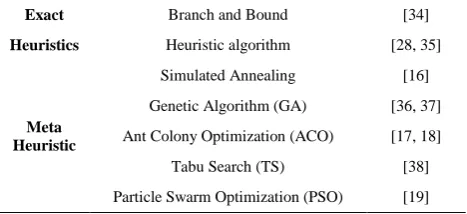
Table 1 shows several articles that used exact, heuristic and meta heuristic algorithms for solving mixed-model assembly line balancing problems.
According to the nature of task times, ALBP is classified into two classes: deterministic and stochastic. Most of the researches in the field of Assembly line balancing assumed that the task times are deterministic [27], but in a realistic manufacturing environment, the task time may be random due to worker fatigue, low skill levels, job dissatisfaction, poorly maintained equipment, defects in raw materials, etc. [28]. Hence, verifying stochastic task time in assembly line balancing will be necessary. There are several papers that investigated stochastic task times for assembly line balancing. For example, Tiacci [29] presented an event and object-oriented simulator for assembly lines. His tool, developed in Java, was capable to simulate mixed model assembly lines, with stochastic task times, parallel stations, fixed scheduling sequences, and buffers within workstations. Also, Cakir et al. [25] proposed an algorithm, based on simulated annealing for multi-objective optimization of a single-model stochastic assembly line balancing problem with parallel stations. The objectives of their paper were (1) minimization of the smoothness index and (2) minimization of the design cost.
A good measure of assembly line balancing in stochastic condition is system reliability. So, there are some papers in this field such as literatures [30-33]. Reliability can be used as a good index when there is uncertainty or probabilistic parameters for system. One of these uncertainties, probabilistic or feasible parameters may be processing times when human involve in assembly line. The reliability of a system with stochastic task time can be defined as a probability that there is no bottleneck in a system.
To the best of our knowledge and literature review, there is no paper that investigated stochastic mixed model assembly line balancing problem according to system reliability, weighted line efficiency and weighted smoothness index, simultaneously. So, this field can be a good area for developing and in this paper we focus on this gap.
TABLE 1. Exact, heuristic and meta heuristics for solving mixed-model ALBP
Exact Branch and Bound [34]
Heuristics Heuristic algorithm [28, 35]
Meta Heuristic
Simulated Annealing [16]
Genetic Algorithm (GA) [36, 37]
Ant Colony Optimization (ACO) [17, 18]
Tabu Search (TS) [38]
Particle Swarm Optimization (PSO) [19]
For this purpose, we propose an SA algorithm for solving mixed model assembly line balancing with stochastic processing time that minimizes weighted smoothness index and maximizes system reliability and weighted line efficiency. The rest of this paper is structured as follows. Section 2 provides some basic concepts about the standard simulated annealing algorithm and weighted sum method for solving multi-objective mathematical models. Problem definition and the proposed simulated annealing algorithm are presented in Section 3. Numerical example and numerical experiments are given in Sections 4 and 5. Finally, Section 6 is devoted to conclusions and recommendations for future research.
2. BASIC CONCEPTS
In this section, we introduce the SA algorithm and weighted sum method for solving multi-objective problems.
2. 1. The Standard Simulated Annealing Algorithm The Simulated Annealing algorithm is a random search optimization technique that got its existence from the physical annealing of solid metal.
As Simulated Annealing starts, an initial solution is generated and used as the first current solution. A control parameter (T), is specified analogous to the annealing temperature. This temperature is systematically decreased according to a cooling rate. As the temperature drops, neighboring solutions to the current solution are found. If the objective function value is superior to that of the current solution, the neighboring solution becomes the new current solution. If the neighboring solution provides an objective function value inferior to that of the current solution, the neighboring solution may still become the current solution if a certain acceptance criterion is met. A distinctive feature of Simulated Annealing is that inferior solutions are sometimes accepted as the current solution to prevent getting trapped in local optima. Through the occasional acceptance of inferior solutions which meet the acceptance criteria, the search moves to a different location on the continuum of feasible solutions in an effort to reach the global optimum. The process of finding neighboring solutions and accepting these as current solutions if acceptance criteria are met is repeated according to the cooling pattern until some stopping criteria is met [39].
of this method is given below [40]:
𝑀𝑖𝑛 𝐹(𝑋) = ∑𝑀𝑚=1𝑤𝑚𝑓𝑚(𝑋)
𝑠𝑢𝑏ject to: 𝐺(𝑋) = [𝑔1(𝑋), 𝑔2(𝑋), … , 𝑔𝐽(𝑋)] ≥ 0
𝐻(𝑋) = [ℎ1(𝑋), ℎ2(𝑋), … , ℎ𝐾(𝑋)] = 0 𝑥𝑖(𝐿)≤ 𝑥𝑖≤ 𝑥𝑖
(𝑈)
, 𝑖 = 1,2, … , 𝑁
(1)
where, the objectives are normalized and wm∈[0, 1] is the weight of the mth objective function.
It is usual practice to choose weights such that ∑𝑀𝑖=1𝑊𝑚=
1.
3. PROBLEM DEFINITION
In this section the problem assumptions and the proposed algorithm for mixed model assembly line balancing problem with stochastic processing time for maximizing the weighted line efficiency (minimizing the number of stations), minimizing the smoothness index and maximizing the system reliability are introduced.
3. 1. Problem Assumptions The assumptions of this problem are given as follows:
1. The required time to do Task j is stochastic, and it has a Normal distribution with mean tj and standard deviation j.
2. Precedence diagrams of different product models are known, and a task cannot be performed until all its predecessors have been completed
3. Common tasks among different product models exist. A task completion time can be different from one model to another.
4. Parallel stations and work-in-process inventories are not allowed.
5. Tasks must be processed only once in each cycle and each task can be assigned to only one station.
6. Stations are arranged in a simple straight assembly line.
7. The maximum cycle time is given.
8. All line workers are paid the same hourly rate and each station is manned by one worker.
9. Demand rate is deterministic.
3. 2. The Proposed SA Algorithm In the proposed SA algorithm, the temperature of each iteration is decreased by using the following relation until the final temperature is reached
TC+1= α. TC (2)
where, α, TC and TC+1 are cooling rate, current temperature and next temperature, simultaneously. Initial solution generation, neighborhood move and structure of building a feasible solution in the algorithm are given as follows.
3. 2. 1. Initial Solution Generation Each solution in proposed algorithm is a string of integer numbers.
The initial solution of proposed algorithm is shown in a list that is named priority list (PL) and the length of this list is as equal as the number of tasks. The position and the value of the position of this list are important. At the first time, this list generates randomly.
For example if there are 6 tasks in an assembly line, an initial and random priority list can be shown with PL= {2, 1, 4, 5, 3, 6}. It means that Task 2 has the highest priority value and Task 6 has the lowest priority value. For creating a feasible solution, the assignable tasks that satisfy the precedence constraints are assigned to the station according to their priority values. Then, the set of assignable tasks is updated. Also, when the current station is loaded maximally, it is closed and the next station is opened. This process continues until all tasks are assigned to the stations.
3. 2. 2. Neighborhood Move In the proposed algorithm, a neighbor solution of priority list is generated by interchanging 2 or 3 tasks randomly with a probability of 0.5 which is shown in Figure 1. If the generate random value is less than or equal to 0.5, interchanging 2 tasks will be selected, otherwise, interchanging 3 tasks method will be happened.
3. 2. 3. Building a Feasible Solution In the procedure of building a feasible solution, the stations have been considered successively. Before the presentation of the procedure of building a feasible solution and calculating the objective functions, it is necessary to introduce the following notations:
i, h, p, r: Task indices j: Station index m: Product model M: Set of product models
P(i): Set of immediate predecessors of Task i tim: Operation time of Task i for model m tfim: Finish time of Task i for model m NS: Number of stations
NM: Number of models NT: Number of tasks SAT: Set of assignable tasks
mWLNS: The station load including unavoidable idle times on the station for all m∈M
TLNS: The set of tasks which are assigned to the station C: Maximum cycle time
Ct: Trial cycle time Cmin: Minimum cycle time
The Procedure of building a solution is as follows: 1. Set NS = 1, mWLNS=0 for all m∈M.
2. Determine SAT (SAT = {i | (all p∈P (i) have already been assigned or P(i) = {Ø}) and Task i has not been assigned}). If SAT= {Ø}, then go to Step 6.
3. Sort the tasks in SAT in increasing order of priority value of tasks in PL.
4. Assign the first Task h in SAT for which;
4.1. If thm+mWLNS ≤ Ct and thm+tfrm≤ Ct (tfrm=max {tfpm| p∈P(h) have already been assigned to the station}) for all m∈M, then assign Task h to the station; TLNS=TLNS+{h}, and set tfhm=max{(thm+mWLNS), (thm + tfrm)} for all m∈M. Set mWLNS=tfhml for all m∈M and go to Step 2; otherwise go to Step 5.
5. If none of these tasks in SAT could be assigned at the station, then open a new station. If TLNS≠{Ø} then NS=NS+1, mWLNS = 0 for all m∈M, and go to Step 2. 6. Stop.
The trial cycle time (Ct) starts from minimum feasible cycle time in the above procedure. It is as follows: Cmin=max[19] i=1, 2,…, NT and m=1,2, …, NM} After creating a feasible solution with this trial cycle time, the objective function according to Section 3.2.4 is calculated. Then the trial cycle time is increased by one unit and the above procedure is repeated until Ct≤C.
3. 2. 4. Objective Function The objectives of the proposed algorithm for mixed model assembly line balancing with stochastic task time for the given maximum cycle time are as follows:
1. Maximization of the weighted line efficiency. It is equivalent to minimize the number of stations or minimizing the line length or the number of operators. Considering the mixed-model nature of the problem, the weighted line efficiency (WLE) is calculated as follows for a given line balance [17]:
WLE=(∑mϵMqm(∑iϵItim)
C.NS ).100 (3)
where, qm is the overall proportion of the number of units of model m. qm is computed by the following equation where Dm denotes the demand, over the planning horizon, for model m.
qm= Dm
∑mϵMDm (4)
2. Minimizing the weighted smoothness index. This index permits decreasing the workload difference between stations where WLmax is the maximum station time.
WSI = √∑mϵMqm.(∑ (jϵJmWLj−WLmax)2)
NS (5)
3. Maximizing the reliability of system.
In this system, the reliability of each station means the probability that the station is not a bottleneck according to stochastic task time. Thus, reliability of jth
workstation (Rj) with trial cycle time Ct can be defined as follows:
Rj= P(∑NTi=1∑NMm=1 qm.timj≤ Ct)=
P((∑NTi=1∑m=1NM qm.timj)−E(∑NTi=1∑NMm=1qm.timj) √∑ ∑NM
m=1qm.2 var(timj) NT
i=1
≤Ct−E(∑NTi=1∑NMm=1qm.timj) √∑ ∑NM
m=1qm.2 var(timj) NT
i=1
) =
P(Z ≤ Ct−(∑NTi=1∑NMm=1qm.μimj) √∑ ∑NM
m=1qm.2var(timj) NT
i=1
)
(6)
Since we have an arrangement of N stations in series, the reliability of the assembly line (RAL) can be expressed as:
RAL= ∏Nj=1Rj (7)
According to the weighted sum method, the objective function of the proposed approach is as follow:
Minimize E = W1( WLE0
WLE) + W2( WSI WSI0) + W3(
RAL0
RAL) (8)
where, WLE0, WSI0 and RAL0 are the objective function values obtained from the initial solution and W1, W2 and W3 are the weights of objectives in the weighted sum method. In this paper, the weight of each objective function is 1.3.
3. 3. Simple Lower Bound In this section, we propose a simple lower bound on the minimal number of stations for mixed model stochastic assembly line balancing. This lower bound is as follows:
LB = ⌈∑NMm=1∑NTi=1qmtim Ct ⌉
(9)
(⌈x⌉ denotes the smallest integer not being smaller than x).
3. 4. Parameter Settings In the meta heuristic algorithms, choosing the best combination of the parameters can intensify the search process and prevent premature convergence.
In this paper, the Taguchi (1986) method is used for the best parameter selections.
Three levels are selected for each parameter of the SA algorithm. They are shown in Table 2.
The Taguchi method uses orthogonal arrays for decreasing the number of experiments for parameter settings. These arrays are presented in Table 3.
TABLE 2. Factors and their levels
Factor Initial temperature
Final temperature
Length of the
Markov chain Cooling rate
level 1 2 3 1 2 3 1 2 3 1 2 3
value 50 100 150 0.5 1 2 5 10 n* 0.9 0.95 0.99
TABLE 3. The orthogonal arrays for the proposed approach
Test Initial Temperature
Final Temperature
Length 0f the Markov
Chain
Cooling Rate
1 1 1 1 1
2 1 2 2 2
3 1 3 3 3
4 2 1 2 3
5 2 2 3 1
6 2 3 1 2
7 3 1 3 2
8 3 2 1 3
9 3 3 2 1
It shows nine tests are necessary to select the best value for each parameter.
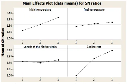
Each test is run four times, and the average of the objective function is obtained to estimate the (SN) ratio. In the Taguchi method, the S/N ratio is as follows: 𝑆𝑁 = −10log (1𝑛∑𝑛 (𝑜𝑏𝑗𝑒𝑐𝑡𝑖𝑣𝑒 𝑓𝑢𝑛𝑐𝑡𝑖𝑜𝑛)2)
𝑖=1 (10)
Each level which has the maximum SN ratio is the best one.
According to Figure 2, the best level of each parameter is reported in Table 4.
4. NUMERICAL EXAMPLE
We illustrate the proposed algorithm by using a nine-task and two-model example problem. Expected nine-task times and their variances are generated randomly.
Figure 2. The mean SN ratio plot for the selected levels of each factor
TABLE 4. Factors and their levels
Factor Initial Temperature
Final Temperature
Length of the Markov
Chain
Cooling Rate
level 3 3 3 3
value 150 2 n* 0.99
The required data such as Expected task time (μ(i)) and variance of task time ( i2) of this example are given in Table 5. The maximum cycle time of this problem is 9.
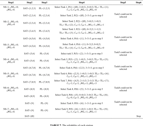
The overall proportion of the number of units of model A and B is o.5. So, qA=qB=50%. The initial random solution (priority list) constructed as: PL = {1, 2, 3, 4, 5, 6, 7, 8, 9}. The procedure of creating the initial line balance is shown in Table 6. The assignment of tasks to the stations and the reliability of each station are presented in Table 7. It shows there are seven stations in system with initial trial cycle time=3. The reliability of station 5 is lower than the others. It can show the importance of this station because it has this ability that will be a bottleneck. The objective function values of WLE, WSI, RLA and E of the initial line balance are 59.524%, 1.711, 0.389 and 1, respectively.
In the next step, a new neighbor solution is generated by interchanging 2 or 3 tasks randomly with a probability of 0.5. These steps are repeated until the final temperature is met. Then, the trial cycle time is increased by one unit and the above procedure is repeated until Ct≤9.
In this problem, according to several preliminary experiments we selected initial temperature, final temperature and cooling rate as 100, 1 and 0.95, respectively.
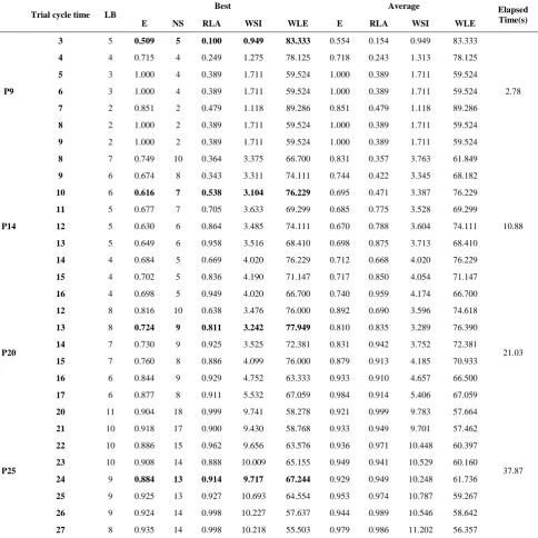
We run this algorithm 5 times with PC 2.2 GHz CPU and 1 GB of RAM. The best and the average results of these iterations are presented in Table 8.
The best function value in 5 iterations with different initial random solution for this problem is 0.509. The number of stations is 5 and the RLA, WSI and WLE are 0.100, 0.949 and 83.333, respectively.
5. NUMERICAL EXPERIMENT
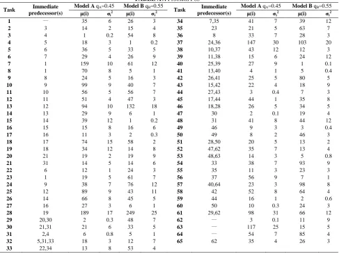
In order to assess the effectiveness of the proposed algorithm, a set of standard test problems (P9, P14, P20, P25, P30, P39, P47 and P65) are solved.
TABLE 5. Data of the example problem
Task Immediate Predecessors
Model A Model B
μ(i) i2 μ(i) i2
1 __ 2 0.5 0 0
2 __ 3 0.8 1 0.3
3 __ 0 0 1 0.3
4 1 3 0.8 0 0
5 2 1 0.3 3 0.8
6 2,3 1 0.3 1 0.3
7 4,5 2 0.5 2 0.5
8 5 0 0 3 0.8
TABLE 6. Building the initial line balance
Step1 Step2 Step3 Step4 Step5 Step6
NS=1; AWL1=0; BWL1=0.
SAT={1,2,3} PL={1,2,3} Select Task 1, P(1) ={Ø}; 2+0≤3;, 0+0≤3; TL1= TL1+{1};
tf
1A=2, tf1B=0, AWL1=2, BWL1=0
SAT={2,3,4} PL={2,3,4} Select Task 2, P(2) ={Ø}; 2+3>3; go to step 5 Task2 could not be selected
NS=2, AWL2=0; BWL2=0
SAT={2,3,4} PL={2,3,4} Select Task 2, P(2) ={Ø}; 3+0≤3; 1+0≤3; TL2= TL2+{2}; tf2A=3, tf2B=1, AWL2=3, BWL2=1
SAT={3,4,5} PL={3,4,5} Select Task 3, P(3) ={Ø}; 0+3≤3; 1+1≤3; TL2= TL2+{3}; tf3A=3, tf3B=2, AWL2=3, BWL2=2
SAT={4,5,6} PL={4,5,6} Select Task 4, P(4) ={1}; 3+3>3; go to step 5 Task4 could not be selected
NS=3; AWL3=0; BWL3=0.
SAT={4,5,6} PL={4,5,6} Select Task 4, P(4) ={1}; 0+3≤3; 0+0≤3; TL3= TL3+{4}; tf4A=3, tf4B=0, AWL3=3, BWL3=0
SAT={5,6} PL={5,6} Select task 5, P(5) ={2}; 1+3>3; go to step 5 Task5 could not be selected
NS=4, AWL4=0;
BWL4=0 SAT={5,6} PL={5,6}
Select Task 5, P(5) ={2}; 1+0≤3;, 3+0≤3; TL4= TL4+{5};
tf
5A=1, tf5B=3, AWL4=1, BWL4=3
SAT={6,7,8} PL={6,7,8} Select Task 6, P(6) ={2,3}; 3+3>3; go to step 5 Task6 could not be selected
NS=5; AWL5=0; BWL5=0.
SAT={6,7,8} PL={6,7,8} Select Task 6, P(6) ={2,3}; 1+0≤3; 1+0≤3; TL5= TL5+{6};
tf
6A=1, tf6B=1, AWL5=1, BWL5=1
SAT={7,8,9} PL={7,8,9} Select Task 7, P(6) ={4,5}; 2+1≤3; 2+1≤3; TL5= TL5+{7}; tf7A=3, tf7B=3, AWL5=3, BWL5=3
NS=6; AWL6=0; BWL6=0.
SAT={8,9} PL={8,9} Select Task 8, P(8) ={5}; 3+3>3; go to step 5 Task8 could not be selected
SAT={8,9} PL={8,9} Select Task 8, P(8) ={5}; 0+0≤3; 3+0≤3; TL6= TL6+{8}; tf
8A=0, tf8B=3, AWL6=0, BWL6=3
SAT={9} PL={9} Select Task 9, P(9) ={6}; 1+3>3; go to step 5 Task9 could not be selected
NS=7; AWL7=0;
BWL7=0. SAT={9} PL={9}
Select Task 9, P(9) ={6}; 1+0≤3; 1+0≤3; TL7= TL7+{9};
tf
9A=1, tf9B=1, AWL7=1, BWL7=1
SAT={Ø} Stop
TABLE 7. The reliability of each station
Station 1 2 3 4 5 6 7
Tasks 1 2,3 4 5 6,7 8 9
∑ ∑𝑵𝑴
𝒎=𝟏 𝒒𝒎.𝝁𝒊𝒎𝒋 𝑵𝑻
𝒊=𝟏 1 2.5 1.5 2 3 1.5 1
∑ ∑𝑵𝑴
𝒎=𝟏 𝒒𝒎.𝟐𝒗𝒂𝒓(𝒕𝒊𝒎𝒋) 𝑵𝑻
𝒊=𝟏 0.125 0.35 0.2 0.275 0.4 0.2 0.15
RLj 1.0000 0.801 0.9996 0.9717 0.5 0.9996 1.0000
The details of these problems are illustrated in Appendix. The parameters of the proposed algorithm are as follows:
T0=100; T0=1; r=0.95 and the length of Markov chain is as equal as the number of tasks. Each problem is solved five times with initial random solution and the
TABLE 8. Comparison results for the small-sized test problems.
Trial cycle time LB
Best Average Elapsed
Time(s)
E NS RLA WSI WLE E RLA WSI WLE
P9
3 5 0.509 5 0.100 0.949 83.333 0.554 0.154 0.949 83.333
2.78
4 4 0.715 4 0.249 1.275 78.125 0.718 0.243 1.313 78.125
5 3 1.000 4 0.389 1.711 59.524 1.000 0.389 1.711 59.524
6 3 1.000 4 0.389 1.711 59.524 1.000 0.389 1.711 59.524
7 2 0.851 2 0.479 1.118 89.286 0.851 0.479 1.118 89.286
8 2 1.000 2 0.389 1.711 59.524 1.000 0.389 1.711 59.524
9 2 1.000 2 0.389 1.711 59.524 1.000 0.389 1.711 59.524
P14
8 7 0.749 10 0.364 3.375 66.700 0.831 0.357 3.763 61.849
10.88
9 6 0.674 8 0.343 3.311 74.111 0.744 0.422 3.345 68.182
10 6 0.616 7 0.538 3.104 76.229 0.695 0.471 3.387 76.229
11 5 0.677 7 0.705 3.633 69.299 0.685 0.775 3.528 69.299
12 5 0.630 6 0.864 3.485 74.111 0.670 0.788 3.604 74.111
13 5 0.649 6 0.958 3.516 68.410 0.698 0.875 3.713 68.410
14 4 0.684 5 0.669 4.020 76.229 0.712 0.668 4.020 76.229
15 4 0.702 5 0.836 4.190 71.147 0.717 0.850 4.054 71.147
16 4 0.698 5 0.949 4.020 66.700 0.740 0.959 4.174 66.700
P20
12 8 0.816 10 0.638 3.476 76.000 0.892 0.690 3.596 74.618
21.03
13 8 0.724 9 0.811 3.242 77.949 0.810 0.835 3.289 76.390
14 7 0.730 9 0.925 3.525 72.381 0.831 0.942 3.752 72.381
15 7 0.760 8 0.886 4.099 76.000 0.879 0.913 4.185 70.933
16 6 0.844 9 0.929 4.752 63.333 0.933 0.910 4.657 66.500
17 6 0.877 8 0.911 5.532 67.059 0.984 0.914 5.406 67.059
P25
20 11 0.904 18 0.999 9.741 58.278 0.921 0.999 9.783 57.664
37.87
21 10 0.918 17 0.900 9.430 58.768 0.933 0.949 9.701 57.462
22 10 0.886 15 0.962 9.656 63.576 0.936 0.971 10.448 60.397
23 10 0.908 14 0.888 10.009 65.155 0.949 0.941 10.529 60.160
24 9 0.884 13 0.914 9.717 67.244 0.929 0.949 10.248 61.736
25 9 0.925 13 0.927 10.693 64.554 0.953 0.974 10.787 59.267
26 9 0.924 14 0.998 10.227 57.637 0.944 0.989 10.546 58.642
27 8 0.935 14 0.998 10.218 55.503 0.979 0.986 11.202 56.357
The above table shown the proposed algorithm can be as an effective algorithm because the initial objective value (E) was 1 and it decreased the duration of running algorithm. Furthermore, the weighted line efficiency and the reliability of system were increased and the
weighted smoothness index was decreased,
simultaneously. For example, the initial values of WLE, WSI and RLA for each P65 are given as follows: Also, the number of stations found by SA algorithm is compared to LB given in Equation (10).
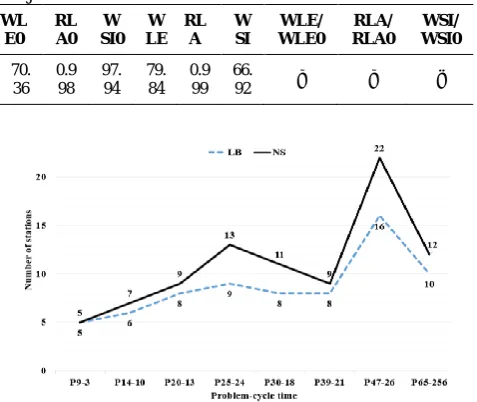
As it can be seen, the proposed SA algorithm performs well throughout on the different problems. Figure 3 shows a comparison between the lower bound and the obtained number of stations by the proposed algorithm. This Figure shows the structure of the problem (predecessors, task times, …) has important effect on the obtained results.
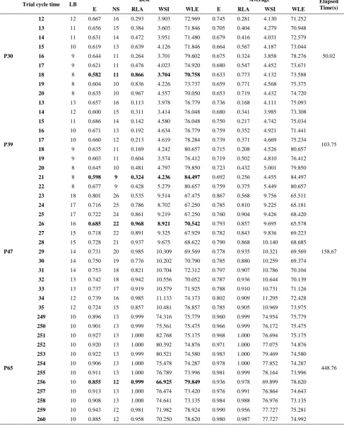
TABLE 9. Computational results for the large-sized test problems
Trial cycle time LB Best Average Elapsed
Time(s)
E NS RLA WSI WLE E RLA WSI WLE
P30
12 12 0.667 16 0.293 3.903 72.969 0.745 0.281 4.130 71.252
50.02
13 11 0.656 15 0.384 3.603 71.846 0.705 0.404 4.279 70.948
14 11 0.631 14 0.472 3.951 71.480 0.679 0.416 4.031 72.579
15 10 0.619 13 0.639 4.126 71.846 0.664 0.567 4.187 73.044
16 9 0.644 11 0.264 3.701 79.602 0.675 0.324 3.858 78.276
17 9 0.621 11 0.476 4.023 74.920 0.680 0.547 4.452 73.671
18 8 0.582 11 0.866 3.704 70.758 0.633 0.773 4.132 73.588
19 8 0.604 10 0.836 4.226 73.737 0.659 0.771 4.568 75.375
20 8 0.635 10 0.967 4.557 70.050 0.653 0.719 4.432 74.720
P39
13 13 0.657 16 0.113 3.978 76.779 0.736 0.168 4.111 75.093
103.75
14 12 0.600 15 0.311 3.414 76.048 0.680 0.341 3.985 73.308
15 11 0.686 14 0.142 4.580 76.048 0.750 0.217 4.742 75.034
16 10 0.671 13 0.192 4.634 76.779 0.759 0.352 4.921 71.441
17 10 0.660 12 0.213 4.619 78.284 0.739 0.371 4.669 75.234
18 9 0.635 11 0.169 4.242 80.657 0.715 0.208 4.526 80.657
19 9 0.603 11 0.604 3.574 76.412 0.719 0.502 4.810 76.412
20 8 0.645 10 0.481 4.797 79.850 0.723 0.432 5.001 79.850
21 8 0.598 9 0.324 4.236 84.497 0.692 0.256 4.455 84.497
22 8 0.677 9 0.428 5.279 80.657 0.759 0.375 5.449 80.657
P47
23 18 0.801 26 0.535 9.514 67.475 0.867 0.568 9.756 65.511
158.67
24 17 0.716 25 0.786 8.702 67.250 0.785 0.810 9.225 65.181
25 17 0.722 24 0.861 9.219 67.250 0.760 0.904 9.426 68.420
26 16 0.685 22 0.968 8.921 70.542 0.793 0.857 9.695 65.578
27 15 0.718 22 0.891 9.325 67.929 0.782 0.843 9.836 69.223
28 15 0.728 21 0.937 9.675 68.622 0.790 0.868 10.140 68.685
29 14 0.731 20 0.985 10.309 69.569 0.778 0.935 10.321 69.569
30 14 0.750 19 0.776 10.202 70.790 0.785 0.880 10.259 69.374
31 14 0.753 18 0.821 10.704 72.312 0.797 0.907 10.786 70.104
32 13 0.742 18 0.942 10.556 70.052 0.787 0.936 10.644 70.139
33 13 0.737 17 0.919 10.579 71.925 0.788 0.910 10.731 71.126
34 12 0.739 16 0.985 11.133 74.173 0.802 0.909 11.295 72.428
35 12 0.724 15 0.857 10.481 76.857 0.785 0.905 10.969 73.975
P65
249 10 0.896 13 0.999 74.316 75.779 0.960 0.999 74.954 75.779
448.76
250 10 0.901 13 0.999 75.561 75.475 0.966 0.999 76.172 75.475
251 10 0.927 13 1.000 82.768 75.175 0.968 1.000 76.694 75.175
252 10 0.920 13 1.000 80.392 74.876 0.971 1.000 77.075 74.876
253 10 0.922 13 0.999 80.521 74.580 0.983 1.000 79.469 74.580
254 10 0.906 13 1.000 75.478 74.287 0.978 1.000 77.852 74.287
255 10 0.911 13 1.000 76.789 73.996 0.981 0.999 78.164 73.996
256 10 0.855 12 0.999 66.925 79.849 0.936 0.978 69.899 78.620
257 10 0.913 13 1.000 76.474 73.420 0.976 0.991 76.864 74.643
258 10 0.908 13 1.000 74.641 73.135 0.984 0.988 76.976 73.135
259 10 0.943 12 0.981 71.982 78.924 0.990 0.956 77.727 75.281
TABLE 10. Comparison between the initial and the best objective functions for P65
WL E0 RL A0 W SI0 W LE RL A W SI WLE/ WLE0 RLA/ RLA0 WSI/ WSI0 70. 36 0.9 98 97. 94 79. 84 0.9 99 66.
92 ↑ ↑ ↓
Figure 3. Comparison between the lower bound and the obtained number of stations
6. CONCLUSION
In this paper, we presented a multi-objective simulated annealing algorithm for mixed-model assembly line balancing with stochastic processing time to maximize the weighted line efficiency (minimizing number of stations), minimizing the weighted smoothness index and maximizing the reliability of system. In this problem maximum cycle time is given. An illustrative example problem is solved by using the proposed algorithm, and numerical experiments are conducted to demonstrate the efficiency of the proposed approach. The results show that the proposed approach obtains good solutions within a short computational time for every test problem because the best result of the objective value (E) in the initial solution was 1 and it decreased in the duration of the proposed algorithm. For further researches the development of this condition for a given number of stations and also using the other meta heuristics may be good subjects.
7. REFERENCES
1. Salveson, M.E., "The assembly line balancing problem",
Journal of Industrial Engineering, Vol. 6, No. 3, (1955),
18-25.
2. Baybars, I., "A survey of exact algorithms for the simple assembly line balancing problem", Management Science, Vol. 32, No. 8, (1986), 909-932.
3. Ghosh, S. and Gagnon, R.J., "A comprehensive literature review and analysis of the design, balancing and scheduling of assembly systems", The International Journal of Production Research, Vol. 27, No. 4, (1989), 637-670.
4. Amen, M., "Heuristic methods for cost-oriented assembly line balancing: A survey", International Journal of Production
Economics, Vol. 68, No. 1, (2000), 1-14.
5. Amen, M., "Cost-oriented assembly line balancing: Model formulations, solution difficulty, upper and lower bounds",
European Journal of Operational Research, Vol. 168, No. 3,
(2006), 747-770.
6. Boysen, N., Fliedner, M. and Scholl, A., "A classification of assembly line balancing problems", European Journal of
Operational Research, Vol. 183, No. 2, (2007), 674-693.
7. Boysen, N., Fliedner, M. and Scholl, A., "Assembly line balancing: Which model to use when?", International Journal
of Production Economics, Vol. 111, No. 2, (2008), 509-528.
8. Becker, C. and Scholl, A., "A survey on problems and methods in generalized assembly line balancing", European Journal of
Operational Research, Vol. 168, No. 3, (2006), 694-715.
9. Hu, S.J., Ko, J., Weyand, L., ElMaraghy, H., Lien, T., Koren, Y., Bley, H., Chryssolouris, G., Nasr, N. and Shpitalni, M., "Assembly system design and operations for product variety",
CIRP Annals-Manufacturing Technology, Vol. 60, No. 2,
(2011), 715-733.
10. Scholl, A. and Becker, C., "State-of-the-art exact and heuristic solution procedures for simple assembly line balancing",
European Journal of Operational Research, Vol. 168, No. 3,
(2006), 666-693.
11. Battaïa, O. and Dolgui, A., "A taxonomy of line balancing problems and their solutionapproaches", International Journal
of Production Economics, Vol. 142, No. 2, (2013), 259-277.
12. Sivasankaran, P. and Shahabudeen, P., "Literature review of assembly line balancing problems", The International Journal
of Advanced Manufacturing Technology, Vol. 73, No. 9-12,
(2014), 1665-1694.
13. Erel, E. and Gokcen, H., "Shortest-route formulation of mixed-model assembly line balancing problem", European Journal of
Operational Research, Vol. 116, No. 1, (1999), 194-204.
14. Karabatı, S. and Sayın, S., "Assembly line balancing in a mixed-model sequencing environment with synchronous transfers",
European Journal of Operational Research, Vol. 149, No. 2,
(2003), 417-429.
15. Kara, Y., Özgüven, C., Seçme, N.Y. and Chang, C.-T., "Multi-objective approaches to balance mixed-model assembly lines for model mixes having precedence conflicts and duplicable common tasks", The International Journal of Advanced
Manufacturing Technology, Vol. 52, No. 5-8, (2011), 725-737.
16. Özcan, U. and Toklu, B., "Balancing of mixed-model two-sided assembly lines", Computers & Industrial Engineering, Vol. 57, No. 1, (2009), 217-227.
17. Simaria, A.S. and Vilarinho, P.M., "2-antbal: An ant colony optimisation algorithm for balancing two-sided assembly lines",
Computers & Industrial Engineering, Vol. 56, No. 2, (2009),
489-506.
18. Yagmahan, B., "Mixed-model assembly line balancing using a multi-objective ant colony optimization approach", Expert
Systems with Applications, Vol. 38, No. 10, (2011),
12453-12461.
19. Chutima, P. and Chimklai, P., "Multi-objective two-sided mixed-model assembly line balancing using particle swarm optimisation with negative knowledge", Computers &
Industrial Engineering, Vol. 62, No. 1, (2012), 39-55.
20. Manavizadeh, N., Hosseini, N.-s., Rabbani, M. and Jolai, F., "A simulated annealing algorithm for a mixed model assembly u-line balancing type-i problem considering human efficiency and just-in-time approach", Computers & Industrial Engineering, Vol. 64, No. 2, (2013), 669-685.
hybrid discrete artificial bee colony algorithm", Journal of
Manufacturing Systems, Vol. 37, (2015), 672-682.
22. Zacharia, P.T. and Nearchou, A.C., "A population-based algorithm for the bi-objective assembly line worker assignment and balancing problem", Engineering Applications of Artificial
Intelligence, Vol. 49, (2016), 1-9.
23. Zhao, X., Hsu, C.-Y., Chang, P.-C. and Li, L., "A genetic algorithm for the multi-objective optimization of mixed-model assembly line based on the mental workload", Engineering
Applications of Artificial Intelligence, Vol. 47, (2016),
140-146.
24. Fattahi, P., Samoei, P. and Zandieh, M., "Simultaneous multi-skilled worker assignment and mixed-model two-sided assembly line balancing", International Journal of
Engineering-Transactions B: Applications, Vol. 29, No. 2, (2016), 211.
25. Cakir, B., Altiparmak, F. and Dengiz, B., "Multi-objective optimization of a stochastic assembly line balancing: A hybrid simulated annealing algorithm", Computers & Industrial
Engineering, Vol. 60, No. 3, (2011), 376-384.
26. Gutjahr, A.L. and Nemhauser, G.L., "An algorithm for the line balancing problem", Management science, Vol. 11, No. 2, (1964), 308-315.
27. Hamta, N., Ghomi, S.F., Jolai, F. and Shirazi, M.A., "A hybrid pso algorithm for a multi-objective assembly line balancing problem with flexible operation times, sequence-dependent setup times and learning effect", International Journal of
Production Economics, Vol. 141, No. 1, (2013), 99-111.
28. Shin, D., "An efficient heuristic for solving stochastic assembly line balancing problems", Computers & Industrial
Engineering, Vol. 18, No. 3, (1990), 285-295.
29. Tiacci, L., "Event and object oriented simulation to fast evaluate operational objectives of mixed model assembly lines problems", Simulation Modelling Practice and Theory, Vol. 24, (2012), 35-48.
30. Suhail, A., "Reliability and optimization considerations in a conveyor-paced assembly line system", The International
Journal of Production Research, Vol. 21, No. 5, (1983),
627-640.
31. Li, J., Alden, J.M. and Rabaey, J.R., "Approximating feeder line reliability statistics with partial data collection in assembly systems", Computers & Industrial Engineering, Vol. 48, No. 2, (2005), 181-203.
32. Iyer, S. and Srihari, K., "Assembly reliability assessment and life estimation for a stacked area array device", Microelectronics
Reliability, Vol. 50, No. 7, (2010), 978-985.
33. Debdip, K. and Dilip, R., "Designing of an assembly line based on reliability approach", An International Journal of
Optimization and Control: Theories & Applications (IJOCTA),
Vol. 1, No. 1, (2011), 45-52.
34. Bukchin, Y. and Rabinowitch, I., "A branch-and-bound based solution approach for the mixed-model assembly line-balancing problem for minimizing stations and task duplication costs",
European Journal of Operational Research, Vol. 174, No. 1,
(2006), 492-508.
35. Jin, M. and Wu, S.D., "A new heuristic method for mixed model assembly line balancing problem", Computers & Industrial
Engineering, Vol. 44, No. 1, (2003), 159-169.
36. Simaria, A.S. and Vilarinho, P.M., "A genetic algorithm based approach to the mixed-model assembly line balancing problem of type II", Computers & Industrial Engineering, Vol. 47, No. 4, (2004), 391-407.
37. Rabbani, M., Kazemi, S.M. and Manavizadeh, N., "Mixed model u-line balancing type-1 problem: A new approach",
Journal of Manufacturing Systems, Vol. 31, No. 2, (2012),
131-138.
38. Bock, S., "Supporting offshoring and nearshoring decisions for mass customization manufacturing processes", European
Journal of Operational Research, Vol. 184, No. 2, (2008),
490-508.
39. McMullen, P.R. and Frazier, G., "Using simulated annealing to solve a multiobjective assembly line balancing problem with parallel workstations", International Journal of Production
Research, Vol. 36, No. 10, (1998), 2717-2741.
40. Deb, K., "Multi-objective optimization using evolutionary algorithms. John wiley& sons", Inc., New York, NY, (2001).
8. APPENDIX
The details of task times and variances for each problem are presented in Tables A1, A2, A3, A4, A5, A6 and A7.
TABLE A1. Problem P14
Task Immediate predecessor(s)
Model A qA=0.42 Model B qB=0.58
Task Immediate predecessor(s)
Model A qA=0.42 Model BqB=0.58
μ(i) i2 μ(i) i2 μ(i) i2 μ(i) i2
1 --- 0 0 2 0.5 8 4,5 0 0 2 0.5
2 --- 8 4 8 4 9 5 3 1.5 2 0.5
3 1 7 3 7 3 10 6 3 1.5 2 0.5
4 3 7 3 5 2 11 5,6 6 2.5 6 2.5
5 3 2 0.5 2 0.5 12 8 3 1.5 3 1.5
6 3 6 2.5 0 0 13 7, 10, 11 5 2 5 2
7 2,3 4 2 0 0 14 9, 12, 13 4 2 6 2.5
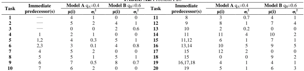
TABLE A2. Problem P20
Task predecessor(s)Immediate Model A μ(i) qA=0.4 Model B qB=0.6 Task predecessor(s) Immediate Model A qA=0.4 Model B qB=0.6
i2 μ(i) i2 μ(i) i2 μ(i) i2
1 ____ 4 1 0 0 11 8 3 0.7 4 1
2 ____ 5 2 4 1 12 9 8 1 7 4
3 ____ 0 0 2 0.6 13 10 2 0.2 0 0
4 1 2 1 0 0 14 11 11 4 10 2
5 1,2 4 0.3 5 1 15 11,12 6 1 7 1
6 2,3 3 0.1 4 0.8 16 13,14 10 5 9 5
7 4 5 2 0 0 17 15 12 2 0 0
8 5 5 1 5 1 18 15 0 0 9 2
9 6 7 0.5 8 0.7 19 16,17,18 4 1 4 1
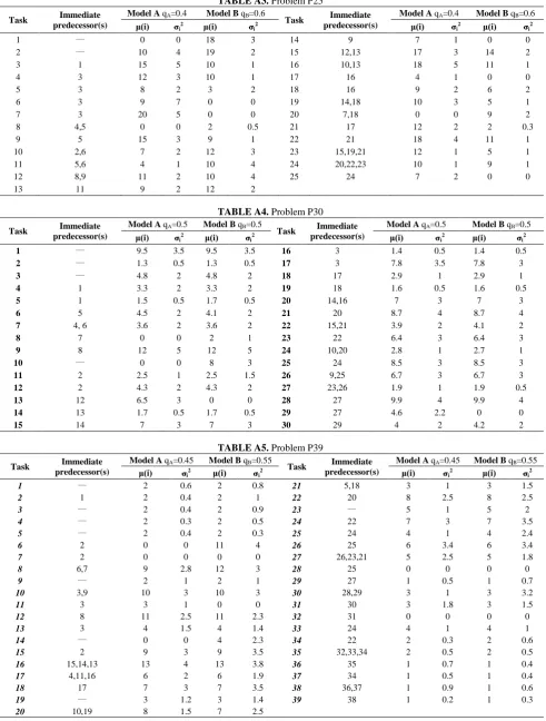
TABLE A3. Problem P25
Task Immediate predecessor(s)
Model A qA=0.4 Model B qB=0.6
Task Immediate predecessor(s)
Model A qA=0.4 Model B qB=0.6
μ(i) i2 μ(i) i2 μ(i) i2 μ(i) i2
1 ___ 0 0 18 3 14 9 7 1 0 0
2 ___ 10 4 19 2 15 12,13 17 3 14 2
3 1 15 5 10 1 16 10,13 18 5 11 1
4 3 12 3 10 1 17 16 4 1 0 0
5 3 8 2 3 2 18 16 9 2 6 2
6 3 9 7 0 0 19 14,18 10 3 5 1
7 3 20 5 0 0 20 7,18 0 0 9 2
8 4,5 0 0 2 0.5 21 17 12 2 2 0.3
9 5 15 3 9 1 22 21 18 4 11 1
10 2,6 7 2 12 3 23 15,19,21 12 1 5 1
11 5,6 4 1 10 4 24 20,22,23 10 1 9 1
12 8,9 11 2 10 4 25 24 7 2 0 0
13 11 9 2 12 2
TABLE A4. Problem P30
Task Immediate predecessor(s)
Model A qA=0.5 Model B qB=0.5
Task Immediate predecessor(s)
Model A qA=0.5 Model B qB=0.5
μ(i) i2 μ(i) i2 μ(i) i2 μ(i) i2
1 ___ 9.5 3.5 9.5 3.5 16 3 1.4 0.5 1.4 0.5
2 ___ 1.3 0.5 1.3 0.5 17 3 7.8 3.5 7.8 3
3 ___ 4.8 2 4.8 2 18 17 2.9 1 2.9 1
4 1 3.3 2 3.3 2 19 18 1.6 0.5 1.6 0.5
5 1 1.5 0.5 1.7 0.5 20 14,16 7 3 7 3
6 5 4.5 2 4.1 2 21 20 8.7 4 8.7 4
7 4, 6 3.6 2 3.6 2 22 15,21 3.9 2 4.1 2
8 7 0 0 2 1 23 22 6.4 3 6.4 3
9 8 12 5 12 5 24 10,20 2.8 1 2.7 1
10 ___ 0 0 8 3 25 24 8.5 3 8.5 3
11 2 2.5 1 2.5 1.5 26 9,25 6.7 3 6.7 3
12 2 4.3 2 4.3 2 27 23,26 1.9 1 1.9 0.5
13 12 6.5 3 0 0 28 27 9.9 4 9.9 4
14 13 1.7 0.5 1.7 0.5 29 27 4.6 2.2 0 0
15 14 7 3 7 3 30 29 4 2 4.2 2
TABLE A5. Problem P39
Task Immediate predecessor(s)
Model A qA=0.45 Model B qB=0.55
Task Immediate predecessor(s)
Model A qA=0.45 Model B qB=0.55
μ(i) i2 μ(i) i2 μ(i) i2 μ(i) i2
1 ___ 2 0.6 2 0.8 21 5,18 3 1 3 1.5
2 1 2 0.4 2 1 22 20 8 2.5 8 2.5
3 ___ 2 0.4 2 0.9 23 ___ 5 1 5 2
4 ___ 2 0.3 2 0.5 24 22 7 3 7 3.5
5 ___ 2 0.4 2 0.3 25 24 4 1 4 2.4
6 2 0 0 11 4 26 25 6 3.4 6 3.4
7 2 0 0 0 0 27 26,23,21 5 2.5 5 1.8
8 6,7 9 2.8 12 3 28 25 0 0 0 0
9 ___ 2 1 2 1 29 27 1 0.5 1 0.7
10 3,9 10 3 10 3 30 28,29 3 1 3 3.2
11 3 3 1 0 0 31 30 3 1.8 3 1.5
12 8 11 2.5 11 2.3 32 31 0 0 0 0
13 3 4 1.5 4 1.4 33 24 4 1 4 1
14 ___ 0 0 4 2.3 34 22 2 0.3 2 0.6
15 2 9 3 9 3.5 35 32,33,34 2 0.5 2 0.5
16 15,14,13 13 4 13 3.8 36 35 1 0.7 1 0.4
17 4,11,16 6 2 6 1.9 37 34 1 0.5 1 0.4
18 17 7 3 7 3.5 38 36,37 1 0.9 1 0.6
19 ___ 3 1.2 3 1.4 39 38 1 0.2 1 0.3
TABLE A6. Problem P47
Task Immediate
predecessor(s)
Model A qA=0.45 Model B qB=0.55
Task Immediate
predecessor(s)
Model A qA=0.45 Model B qB=0.55
μ(i) i2 μ(i) i2 μ(i) i2 μ(i) i2
1 ____ 23 2 2 0.6 25 24 6 2 11 2
2 6 20 3 5 1 26 25 9 1 7 3
3 6 2 0.2 9 2 27 6 7 3 8 1
4 6 6 1 7 0.3 28 20,21 4 1 14 4
5 ____ 14 2 11 4 29 23 3 0.4 19 6
6 1 22 1 23 5 30 28 2 0.1 11 1
7 6 1 0.1 2 0.1 31 23,27 12 2 15 0.5
8 5,6 7 1 6 2 32 31 13 3 4 0.1
9 6 4 2 8 4 33 34 1 0.4 3 1
10 12 8 1 7 1 34 ____ 5 2 2 0.4
11 6 12 4 11 3 35 34 4 3 8 0.2
12 16 9 2 14 5 36 6,33,35 13 6 6 1
13 16 7 1 18 6 37 7 18 5 19 0.5
14 16 3 1 3 0.1 38 37 20 8 15 1
15 6 11 3 1 0.3 39 6 8 0.8 3 0.4
16 15 20 6 6 2 40 7,41 11 5 7 0.3
17 7,9 2 0.8 4 1 41 ____ 17 8 1 0.1
18 17 9 3 5 0.5 42 ____ 3 0.4 8 3
19 6 7 1 11 3 43 7,36 9 5 9 2
20 17 4 1 9 1 44 36,42 7 3 10 2
21 17 3 0.5 4 0.6 45 44 17 3 20 5
22 17 7 0.2 6 2 46 45 14 4 3 0.3
23 28 11 3 2 0.4 47 44 11 5 3 0.1
24 23 5 2 1 0.1
TABLE A7. Problem P65
Task Immediate predecessor(s)
Model A qA=0.45 Model B qB=0.55
Task Immediate predecessor(s)
Model A qA=0.45 Model B qB=0.55
μ(i) i2 μ(i) i2 μ(i) i2 μ(i) i2
1 ___ 35 6 26 3 34 7,35 41 7 39 12
2 3 14 2 15 4 35 23 21 5 63 7
3 4 1 0.2 54 8 36 8 33 7 28 3
4 5 18 3 1 0.2 37 24,36 147 30 103 20
5 6 36 5 33 5 38 10,37 43 12 12 3
6 7 29 4 26 9 39 11,38 15 6 24 12
7 1 159 10 61 12 40 25,39 27 9 1 0.1
8 1 70 8 5 1 41 13,40 4 1 5 0.4
9 8 24 5 16 3 42 26,41 25 5 80 5
10 9 99 9 40 7 43 15,42 22 4 18 9
11 10 56 5 56 7 44 27,43 3 0.4 7 3
12 11 51 4 47 3 45 17,44 44 1 35 8
13 12 94 10 132 18 46 18,28 26 5 34 5
14 13 29 9 6 1 47 30 2 0.1 19 4
15 14 39 12 1 0.2 48 31 41 8 44 12
16 15 15 8 16 6 49 46 9 3 3 0.4
17 16 11 3 2 0.3 50 49 8 2 46 3
18 17 74 15 58 2 51 28,50 20 5 13 2
19 18 34 12 14 8 52 47,62 35 7 13 4
20 21 19 2 19 9 53 48,63 14 3 5 0.8
21 31 14 5 14 6 54 33 38 7 93 9
22 6 12 1 24 3 55 35 11 3 23 3
23 1 19 5 61 7 56 37 56 9 7 1
24 9 38 7 76 12 57 40,64 23 3 98 8
25 12 89 9 43 11 58 42 52 8 64 4
26 14 66 8 45 5 59 44 16 1 2 0.6
27 16 27 3 6 1 60 50 10 0.3 24 3
28 19 189 17 249 25 61 29,62 98 31 66 12
29 20,30 2 0.3 48 7 62 ___ 3 0.1 11 9
30 21,31 21 6 33 5 63 ___ 117 25 15 5
31 2,4 6 0.8 5 1 64 ___ 54 7 85 4
32 5,31,33 18 3 12 7 65 62 35 4 26 3
Mixed-model Assembly Line Balancing with Reliability
P. Samoueia, V. Khodakaramia, P. Fattahib
a Department of Industrial Engineering, Faculty of Engineering, Bu-Ali Sina University, Hamedan, Iran b Department of Industrial Engineering, Alzahra University, Tehran, Iran
P A P E R I N F O
Paper history: Received 21 June 2016
Received in revised form 14 January 2017 Accepted 02 February 2017
Keywords:
Assembly Line Balancing Reliability
Mixed-model
Stochastic Processing Time Line Efficiency
ديكچ ه
هئارا هب هلاقم نیا ژاتنوم طوطخ سنلااب یارب هفدهدنچ یجیردت دامجنا متیروگلا کی ی
لدم یاه نامز اب یبیکرت یاه
یم یفداصت شزادرپ نامز هک اجنآ زا .دزادرپ
هاگولگ یور تسا نکمم یفداصت یاه لقادح ،دشاب راذگریثات متسیس یاه
یزاس هاگتسیا دادعت ممیزکام و نوزوم یزاسراومه صخاش یزاس لقادح ،طخ نوزوم ییاراک یزاس ممیزکام اب لداعم( اه
یم نانیمطا تیلباق یزاس درکلمع ،تاییزج اب هلئسم کی لح زا سپ .تسا هتفرگ رارق هعلاطم دروم قیقحت نیا رد دشاب
هعومجم کمک هب متیروگلا ارق یبایزرا دروم لئاسم زا یا
هدنهد ناشن تاشیامزآ جیاتن هک تسا هتفرگ ر بوخ درکلمع ی
.تسا یداهنشیپ متیروگلا