University of Mazandaran, Iran http://cjms.journals.umz.ac.ir ISSN: 1735-0611 CJMS.7(1)(2018), 102-112
An effective method for approximating the solution of singular integral equations with Cauchy kernel type
A. Shahsavaran1 and M. Paripour2
1 Faculty of Science, Borujerd Branch, Islamic Azad University,
Borujerd, Iran
2 Faculty of Science, Hamedan University of Technology, Hamedan,
Iran
Abstract. In present paper, a numerical approach for solving Cauchy type singular integral equations is discussed. Lagrange interpolation with Gauss Legendre quadrature nodes and Taylor series expansion are utilized to reduce the computation of integral equations into some algebraic equations. Finally, five examples with exact solution are given to show efficiency and applicability of the method. Also, we give the maximum of computed absolute errors for some examples.
Keywords: Singular integral equation, Cauchy kernel, Lagrange interpolation, Taylor series expansion, Gauss Legendre quadrature nodes.
2000 Mathematics subject classification: 45E05; 45B05; 45E10.
1. Introduction
Singular integral equation has enormous applications in applied prob-lems including fluid mechanics, biomechanics, electromagnetic theory and chemistry applications such as heat conduction, crystal growth and electrochemistry. An integral equation is called a singular integral equa-tion if one or both limits of integraequa-tion become infinite, or if the kernel
1Corresponding author: [email protected]
Received: 13 November 2013 Revised: 1 March 2014 Accepted: 10 September 2015
of the equation becomes infinite at one or more points in the interval of integration. Such equations can not be solved exactly, that is why various approximate methods have been developed and applied(see [1, 2, 4-6, 8-10]). The present paper deals with approximate approach to solve the above mentioned singular integral equation. Our study is based on approximating the solution of the Cauchy singular integral equation by Lagrange interpolation. As will be seen, we may overcome the sin-gularity using truncated Taylor series expansion. We first present the Lagrange interpolation and Taylor series expansion of a function and then we introduce singular integral equations with Cauchy kernel type.
2. Gauss Legendre nodes and weights
Let pn(x) be the Legendre polynomial of degree n on the interval [−1,1]. The nodes for quadrature ordernare given by the roots of the Legendre polynomial pn(x) which occur symmetrically about 0. The Gauss Legendre nodes are
−1< x0< x1< ... < xn−1 < xn<1.
No explicit formulas are known for the points xi, and so they are com-puted numerically. Also, the weightswi are given by
wi=
2
(1−x2i) (p′n(xi))2
= 2(1−x
2 i) (n+ 1)2(p
n+1(xi))2
, i= 0,1, ..., n.
For detail see [7]. Beyer (1987) gave a table of nodes and weights up to n= 16. (see [3])
3. Lagrange interpolation and Taylor series expansion
In this paper, we use the idea of the interpolation by Lagrange func-tions to approximate the solution of the singular integral equafunc-tions. The collocation points for the interpolation formula are Gauss Legendre quadrature nodes. A functionψ(x) may be approximated by using La-grange interpolation as
ψ(x)≃ n
∑
i=0
ψili(x), (3.1)
where,
li(x) = n
∏
j=0,j̸=i
(x−xj xi−xj
Also,li(xj) =δij whereδij is the Kronecker delta, which simply implies that,ψi=ψ(xi).Now with the Taylor series expansion ofψ(y) based on expanding about the given pointx∈(−1,1), we have the Taylor series approximation of ψ(y) in the following form
ψ(y) = p
∑
r=0
ψ(r)(x)
r! (y−x) r+r
p(x)
=ψ(x) + p
∑
r=1
ψ(r)(x)
r! (y−x) r+r
p(x)
≃ψ(x) + p
∑
r=1
ψ(r)(x)
r! (y−x)
r, (3.2)
where,
rp(x) =
ψ(p+1)(ξx)
(p+ 1)! (y−x) p+1,
is called the remainder term or truncation error, and ξx is between y and x.Consequently, from (3.2) we obtain
ψ(y)−ψ(x)≃ p
∑
r=1
ψ(r)(x)
r! (y−x)
r. (3.3)
Now, we consider the following singular integral equation
α(x)ψ(x) +β(x)
∫ 1
−1 ψ(y)
y−xdy=f(x), |x|<1, (3.4)
where, α(x) ̸= 0, β(x) ̸= 0 and α(x), β(x), f(x) ∈ L2[−1,1] are given functions andψ(x) is the unknown function to be determined.
4. Method of the solution
To approximate the integral part of the Eq. (3.4), we may proceed as follows
∫ 1
−1 ψ(y) y−xdy=
∫ 1
−1
ψ(y)−ψ(x) +ψ(x) y−x dy
=
∫ 1
−1
ψ(y)−ψ(x) y−x dy+
∫ 1
−1 ψ(x) y−xdy
=
∫ 1
−1
ψ(y)−ψ(x)
y−x dy+ψ(x)
∫ 1
−1 1 y−xdy
By using (3.3), we can approximate I1(x) as follows
I1(x) =
∫ 1
−1
ψ(y)−ψ(x) y−x dy
≃
∫ 1
−1
∑p r=1
ψ(r)(x)
r! (y−x) r
y−x dy
= ∫ 1 −1 p ∑ r=1
ψ(r)(x)
r! (y−x) r−1dy
= p
∑
r=1
ψ(r)(x) r!
∫ 1
−1
(y−x)r−1dy
= p
∑
r=1
ψ(r)(x)
rr! [(1−x)
r−(−1−x)r], |x|<1, (4.2)
and
I2(x) =
∫ 1
−1 1 y−xdy
= ln
(
1−x 1 +x
)
, |x|<1, (4.3)
by substituting (4.2) and (4.3) into (4.1), we obtain
∫ 1
−1 ψ(y) y−xdy≃
p
∑
r=1
ψ(r)(x)
rr! [(1−x)
r−(−1−x)r]+ψ(x) ln
(
1−x 1 +x
)
, |x|<1.
(4.4) Now, we return back to main problem that is approximating the solution for the following singular integral equation
α(x)ψ(x) +β(x)
∫ 1
−1 ψ(y)
y−xdy=f(x), |x|<1, (4.5)
and for simplicity of notation we set
γ(x) =
∫ 1
−1 ψ(y)
Representation of the functions α(x), β(x), f(x) and ψ(x) in terms of Lagrange function yields
α(x)≃ n
∑
i=0
αili(x), αi =α(xi), (4.7)
β(x)≃ n
∑
i=0
βili(x), βi =β(xi), (4.8)
f(x)≃ n
∑
i=0
fili(x), fi =f(xi), (4.9)
ψ(x)≃ n
∑
i=0
ψili(x), ψi=ψ(xi), (4.10)
by substituting the approximations (4.7)-(4.10) and (4.6) into (4.5), we obtain(
n
∑
i=0
αili(x)
) ( n
∑
i=0
ψili(x)
)
+
( n
∑
i=0
βili(x)
)
γ(x) = n
∑
i=0
fili(x), (4.11)
collocating (4.11) at the same Lagrange interpolation points xj, j = 0,1, ..., n and using the fact thatli(xj) =δij, we obtain
( n
∑
i=0 αiδij
) ( n
∑
i=0 ψiδij
)
+
( n
∑
i=0 βiδij
)
γ(xj) = n
∑
i=0
fiδij, (4.12)
which simply yields
αjψj+βjγ(xj) =fj, j = 0,1, ..., n (4.13)
where
γ(xj) = p
∑
r=1
ψ(r)(xj)
rr! [(1−xj)
r−(−1−x
j)r] +ψjln
(
1−xj 1 +xj
)
.
Equation (4.13) is a system ofn+ 1 linear equations which can be solved forψj, j = 0,1, ..., n; therefore, desired approximation for ψ(x) may be obtained by (3.1).
5. Illustrative Examples
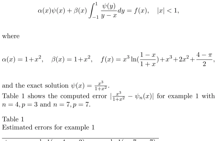
Example 1:
α(x)ψ(x) +β(x)
∫ 1
−1 ψ(y)
y−xdy=f(x), |x|<1,
where
α(x) = 1+x2, β(x) = 1+x2, f(x) =x3ln(1−x 1 +x)+x
3+2x2+4−π 2 ,
and the exact solutionψ(x) = 1+x3x2.
Table 1 shows the computed error |1+x3x2 −ψn(x)| for example 1 with n= 4, p= 3 andn= 7, p= 7.
Table 1
Estimated errors for example 1
t example 1(n=4, p=3) example 1(n=7, p=7)
0.0 9×10⁻² 3×10⁻⁵
0.1 8×10⁻² 5×10⁻⁴
0.2 8×10⁻² 5×10⁻⁴
0.3 7×10⁻² 8×10⁻⁶
0.4 7×10⁻² 6×10⁻⁴
0.5 7×10⁻² 9×10⁻⁴
0.6 6×10⁻² 5×10⁻⁴
0.7 5×10⁻² 1×10⁻⁴
0.8 3×10⁻² 2×10⁻⁴
0.9 1×10⁻² 5×10⁻⁴
Example 2:
α(x)ψ(x) +β(x)
∫ 1
−1 ψ(y)
y−xdy=f(x), |x|<1,
where
and the exact solution ψ(x) =x. In this example, for n= 4 and p = 3 we have
ψ4(x) = 4
∑
i=0
ψili(x)
=.9999999913(−2.719530422x−1.464383670)x(−.6922095881x+.3727336193)
(−.5517668485x+.5000000000) +.9999999913(2.719530422x+ 2.464383670)x
(−.9285580268x+.5000000000)(−.6922095881x+.6272663807) + 0.24×10⁻⁸
(1.103533697x+ 1.000000000)(1.857116054x+ 1.000000000)(−1.857116054x+ 1.000000000)
(−1.103533697x+ 1.000000000) + 1.000000006(.6922095881x+.6272663807)
(.9285580268x+.5000000000)x(−2.719530422x+ 2.464383670) + 1.000000006
(.5517668485x+.5000000000)(.6922095881x+.3727336193)x(2.719530422x−1.464383670)
= 0.2400000000×10⁻⁸+ 0.5×10−8x2+.9999999989x
≃x. (exact solution)
So, maximum error is obtained as
|x−ψ4(x)|< .84×10−8, |x|<1.
Example 3:
α(x)ψ(x) +β(x)
∫ 1
−1 ψ(y)
y−xdy=f(x), |x|<1,
where
α(x) =x2+x+1, β(x) =x2+x+1, f(x) =x5+x4+x3+(x2+x+1)
(
2 3 + 2x
2+x3ln
(
1−x 1 +x
))
and the exact solutionψ(x) =x3.In this example, for n= 4 andp= 3 we have
ψ4(x) = 4
∑
i=0
ψili(x)
=.8211619121(−2.719530422x−1.464383670)x(−.6922095881x+.3727336193)
(−.5517668485x+.5000000000) +.2899491901(2.719530422x+ 2.464383670)x
(−.9285580268x+.5000000000)(−.6922095881x+.6272663807) + 0.25×10⁻⁸
(1.103533697x+ 1.000000000)(1.857116054x+ 1.000000000)(−1.857116054x+ 1.000000000)
(−1.103533697x+ 1.000000000) +.2899492033(.6922095881x+.6272663807)
(.9285580268x+.5000000000)x(−2.719530422x+ 2.464383670) +.8211619249
(.5517668485x+.5000000000)(.6922095881x+.3727336193)x(2.719530422x−1.464383670)
= 0.6×10−9x4+.9999999976x3+ 0.31×10−8x2−0.6×10⁻⁹x+ 0.2500000000×10⁻⁸
≃x3. (exact solution)
So, maximum error is obtained as
|x3−ψ4(x)|< .92×10−8, |x|<1.
Example 4:
α(x)ψ(x) +β(x)
∫ 1
−1 ψ(y)
y−xdy=f(x), |x|<1,
where
α(x) = 2, β(x) = 1, f(x) = 2x4+ 2x3+ 2 3x+x
4ln
(
1−x 1 +x
)
and the exact solutionψ(x) =x4.In this example, for n= 6 andp= 5 we have
ψ6(x) = 6
∑
i=0
ψili(x)
=−.8549618710(−4.817495912x−3.572323476)(−1.840729889x−.7470512979)
x(−.7380329471x+.2995270921)(−.5914922942x+.4386099848)
(−.5268104867x+.5000000000)−.4077446059(4.817495912x+ 4.572323476)
(−2.978974044x−1.209002168)x(−.8715536177x+.3537158087)(−.6742804709x
+.5000000000)(−.5914922942x+.5613900151)−0.6684683406×10⁻¹(1.840729889x
+ 1.747051298)(2.978974044x+ 2.209002168)x(−1.231996982x+.5000000000)
(−.8715536177x+.6462841913)(−.7380329471x+.7004729079)−0.1195×10⁻⁷
(1.053620973x+.9999999996)(1.348560942x+ 1.000000000)(2.463993964x
+.9999999999)(−2.463993964x+.9999999999)(−1.348560942x+ 1.000000000)
(−1.05362097x+.999999999) + 0.668468474×10⁻¹(.738032947x+.7004729079)
(.871553617x+.6462841913)(1.231996982x+.5000000000)x(−2.978974044x
+ 2.209002168)(−1.840729889x+ 1.747051298) +.4077446403(.5914922942x+.5613900151)
(.6742804709x+.5000000000)(.8715536177x+.3537158087)x(2.978974044x
−1.209002168)(−4.817495912x+ 4.572323476) +.8549619302(.5268104867x+.5000000000) (.5914922942x+.4386099848)(.7380329471x+.2995270921)x(1.840729889x
−.7470512979)(4.817495912x−3.572323476)
= 0.32×10⁻⁸x+ 0.24×10−8x2+ 0.18×10−8x3+ 0.9×10−8x5+.999999981x4
−0.51×10−8x6−0.1194999999×10⁻⁸
≃x4. (exact solution)
So, maximum error is obtained as
|x4−ψ6(x)|< .41694999999×10−7, |x|<1.
Example 5:
α(x)ψ(x) +β(x)
∫ 1
−1 ψ(y)
y−xdy=f(x), |x|<1,
where
α(x) = 2, β(x) = 1, f(x) = 2x6+ 2x5+2 3x
3+2 5x+x
6ln
(
1−x 1 +x
)
and the exact solutionψ(x) =x6.In this example, for n= 7 andp= 7 we have
ψ7(x) = 7
∑
i=0
ψili(x)
= 0.392807×10⁻⁷x−0.903043×10−7x2−0.4851×10−6x3+ 0.1453×10−5x5
+ 0.3636×10−6x4+.99999971x6−0.11577436×10−5x7+ 0.683×10⁻⁸
≃x6. (exact solution) So, maximum error is obtained as
|x6−ψ7(x)|< .38858649×10−5, |x|<1.
6. Conclusion
In the present paper, Lagrange functions and truncated Taylor series expansion are applied to solve the Cauchy singular integral equation. Gauss Legendre quadrature nodes were used as the Lagrange interpola-tion points to obtain high accuracy of the approximated soluinterpola-tions. This approach, transforms a singular integral equation to a set of algebraic equations. As was seen, the maximum absolute error was estimated on some examples that show efficiency and applicability of the proposed method. Finally, by some modifications, this method can be extended and applied to integral equations of the form
α(x)ψ(x) +β(x)
∫ 1
−1
k(x, y)ψ(y)
(y−x)α dy=f(x), |x|<1, 0< α≤1.
References
[1] K. E. Atkinson, The numerical solution of integral equations of the second kind, Cambridge University Press, 1997.
[2] C. T. H. Baker, The numerical solution of integral equations, Clarendon Press, Oxford, 1997.
[3] W. H. Beyer, CRC Standard Mathematical Tables, 28th ed. Boca Raton, FL: CRC Press, (1987) 462-463.
[4] L. M. Delves, J. L. Mohammed, Computational methods for integral equa-tions, Cambridge University Press, 1983.
[5] E. A. Galperin, E. J. Kansa, A. Makroglou, S. A. Nelson, Variable trans-formations in the numerical solution of second kind Volterra integral equa-tions with continuous and weakly singular kernels; extensions to Fredholm integral equations, Journal of Computational and Applied Mathematics, 115 (2000) 193-211.
[6] I. Graham, Singularity expansions for the solution of the second kind Fred-holm integral equations with weakly singular convolution kernels, J. Inte-gral Equations, 4 (1982) 1-30.
[8] A. Palamora, Product integration for Volterra integral equation of the second kind with weakly singular kernels, J. Math. Comput. 65 (1996) 1201-1212.