Perceptual Loss for Convolutional Neural Network Based Optical Flow Estimation

2017 2nd International Conference on Software, Multimedia and Communication Engineering (SMCE 2017) ISBN: 978-1-60595-458-5

Perceptual Loss for Convolutional Neural Network

Based Optical Flow Estimation

Zong-qing LU, Xiang ZHU

and Qing-min LIAO

Graduate School at Shenzhen, Tsinghua University, Shenzhen, China

*Corresponding author

Keywords: Convolutional neural networks, Optical flow, Auto-encoder.

Abstract. Convolutional Neural Networks (CNNs) are successfully used in optical flow estimation as learned patch based descriptors. In this work, rather training feature descriptors via CNNs, an end-to-end fully convolutional network, is developed for solving optical flow from a pair of images. Motivated by the success in image transformation tasks, a perceptual loss function is used for training the network for optical flow estimation. We trained a deep convolutional auto-encoder of optical flow field to obtain the high-level representation of motion structures rather than image texture. The perceptual loss function is then defined by high-level features extracted from the pretrained encoder. Conventional variational refinement are not performed. Experiments show the network achieves competitive performance on the challenging MPI Sintel set and Flying Chairs set.

Introduction

Optical flow is topic of great interest in video analysis. By means of its great represent ability of the motion information, optical flow is widely used in object tracking [1], action recognition [2], video stabilization [3] and video frame prediction [4] etc. As a result of illumination changes, deformations, repetitive patterns or occlusions optical flow estimation is a highly ill-posed problem. Though significant progress is made through decades of research, it remains an unsolved problem.

Related Work

Conventional methods [5, 6] estimate the optical flow by minimize a global energy function that is the weighted sum of a data term and a prior term.

𝐸_{𝑔𝑙𝑜𝑏𝑎𝑙} = 𝐸_{𝑑𝑎𝑡𝑎}+ 𝜆 ⋅ 𝐸_{𝑝𝑟𝑖𝑜𝑟} (1) In conditional random field manner, the data term, 𝐸_{𝑑𝑎𝑡𝑎} which penalizes association of dissimilar patches can be treated as unary potentials while the prior term, 𝐸_{𝑝𝑟𝑖𝑜𝑟} which constrains the ill-posed problem can be treated as pairwise potentials [7, 8, 9].

Recently, computer vision tasks, especially per-pixel prediction tasks [10, 11, 12] enjoy the performance boost with deep learning methods. Convolutional neural networks are successfully used in optical flow estimation. One approach [13] for solving optical flow tasks is to train a feedforward convolutional neural network in a supervised manner, using a per-pixel loss function to measure the difference between output and ground-truth flow. Another fashion serve convolutional neural network as a feature descriptor [14, 15]. Patch match method is then employed using these local features extracted by the trained network. Both the end-to-end network approach and the feature descriptor method serve the convolutional neural network as the data term. Thus, post variational refinement [16] is required to provide the absence prior term.

Inspired by these methods, we propose a learned prior term. We first train a variational autoencoder to extract high level feature of motions. Then, a perceptual loss for optical flow is defined by the feature map of different layers from the trained encoder. The perceptual loss is then used to train an end-to-end convolutional neural network for optical flow estimation task. The perceptual loss function takes the role of the pairwise potentials i.e. the prior term in the global energy function.

Contributions

Our contributions are twofold. First, we demonstrate that one can extract motion information using a pretrained variational auto-encoder. Second, we show that applying the encoder to optical flow estimation network without variational refinement achieves competitive performance on different dataset.

Method

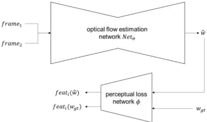
Given a consecutive frame pair 𝑓𝑟𝑎𝑚𝑒₁ and 𝑓𝑟𝑎𝑚𝑒₂, a deep convolutional neural network 𝑁𝑒𝑡_𝛩 is learned to estimate the per-pixel optical flow field 𝑤 = (𝑢, 𝑣) between the two frames, where 𝛩 are the parameters of the network and 𝑢, 𝑣 are the horizontal and vertical components of optical flow, respectively.

Figure 1. The proposed network framework, with two convolutional neural network, one for optical flow estimation, and the other for perceptual loss definition. 𝑓𝑒𝑎𝑡𝑖 is the feature extracted from the 𝑖th level of the perceptual loss network 𝜙.

(Low level loss functions are not shown in this figure.)

The network is then trained using a combined loss functions of a per-pixel loss 𝐿_𝑒𝑝𝑒, a smooth-ness loss 𝐿_{𝑠𝑚𝑜𝑜𝑡ℎ} and a perceptual loss 𝐿_𝜙 defined by a pretrained loss network 𝜙. The loss network remains fixed during the training process. As shown in Figure 1, the optical flow estimation network transforms the concatenated two frames 𝑓𝑟𝑎𝑚𝑒1,2 into optical flow 𝑤̂.

𝑤̂ = 𝑁𝑒𝑡_𝛩(𝑓𝑟𝑎𝑚𝑒_1,2). (2) The network is then trained by stochastic gradient descent method to minimize the combined loss function.

Network Architecture

We flow the FlowNet [13] Simple architecture. The frame pair is concatenated. We first apply a 10-layers convolutional neural network directly to the concatenated input, and then apply 4 sub-pixel convolution layers that upscales the low-resolution optical flow estimation to high-resolution field. Each sub-pixel convolution layer is composed of a normal convolution layer with a pixel shuffling layer. The pixel shuffling [17] layer is a periodic shuffling operator that rearranges the elements of a

popular deconvolution layer. Skip connections between the corresponding layers in the downscale phase and upscale phase is applied to let the low-level information shuttled directly across the net.

Loss Functions

We then define the loss functions. The loss functions are consisted of a per-pixel loss, a smoothness loss and a perceptual loss.

The most common error measure for optical flow evaluation is endpoint error (EPE). Thus, we use the endpoint error as the per-pixel loss.

𝐿_𝑒𝑝𝑒 = 1

𝑁(√(𝑢̂ − 𝑢𝑔𝑡) 2

+ (𝑣̂ − 𝑣_𝑔𝑡)2) (3)

Smoothness prior is a widely-used prior term in conventional methods. Since the loss function is a distance between the estimation and the ground truth, we let the smoothness prior term preserve the edge structure.

𝐿_{𝑠𝑚𝑜𝑜𝑡ℎ} = 1

𝑁(√(∇𝑢̂ − ∇𝑢𝑔𝑡) 2

+ (∇𝑣̂ − ∇𝑣_𝑔𝑡)2) (4)

Finally, we use a loss network 𝜙 to define perceptual loss functions that measure perceptual differences. Let the 𝑓𝑒𝑎𝑡𝑖 denote the output feature map of the 𝑖th layer. The perceptual loss is

defined as,

𝐿𝑝𝑒𝑟𝑐𝑒𝑝𝑡𝑢𝑎𝑙 = ∑ 𝜆𝑖⋅ 1

𝑁(√(𝑓𝑒𝑎𝑡𝑖(𝑤̂) − 𝑓𝑒𝑎𝑡𝑖(𝑤𝑔𝑡)) 2

)

𝑖 (5)

It is trivial to show that the smooth loss defined above is a special case of the perceptual loss. However, the pairwise potentials are much more complicate that the perceptual term should defined by a network. The pretrained loss network used in [10] is for image classification task. The constraint provided contains texture prior of natural image is therefore not suitable for the optical flow estimation problem. A pretrained network extracted motion and structure information while eliminate texture is needed.

Variational Auto-encoder

For optical flow field, there is no label to train a network for classification task. To train a network for high-level motion feature extracting, the network has to learn in an unsupervised manner. Variational auto-encoders [18] make this approach tractable.

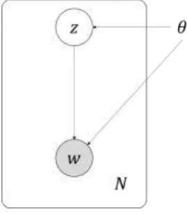
Figure 2. The graphical model.

As shown in Figure 2, the optical flow dataset contains 𝑁 samples of optical flow 𝑤. We assume that a latent random variable 𝑧 which contains the motion information is drawn from a prior distribution 𝑝𝜃(𝑧), then the datum 𝑤(i) is generated from some conditional distribution 𝑝𝜃(𝑤|𝑧). The

input and outputs the parameters 𝜇 and 𝜎 of the prior distribution 𝑝_𝜃(𝑧). After we sample latent variables 𝑧 from the distribution 𝑝_𝜃(𝑧), the decoder reconstructs optical flow back.

Table 1. Variational auto-encoder architecture.

Encoder Decoder

Layer Filter/Stride Layer Filter

Input - Reparametrize -

Conv1 7 × 7 × 64 / 2 Conv6 3 × 3 × 64

Conv2 5 × 5 × 128 / 2 Conv7 3 × 3 × 256

Conv3 3 × 3 × 256 / 2 Pixel Shuffle (2 × 2) -

Conv4 3 × 3 × 512 Conv8 3 × 3 × 32

Conv5_1: 𝜇 Conv5_2: σ

3 × 3 × 2 3 × 3 × 2

Pixel Shuffle (4 × 4) -

Output -

The variational auto-encoder is trained by the loss function defined as the sum of the squared error between the input optical flow and generated field and the Kullback-Liebler (KL) divergence between the distribution created by the encoder and the prior distribution.

𝐿_𝑉𝐴𝐸 = ‖𝑤 − 𝑤̂‖₂+ 𝐾𝐿(𝑞(𝑧|𝑤)||𝑝(𝑧)). (6) To train the variational auto-encoder with backprop method, reparametrize trick [18] is used.

Experiments

We use the image from Flying Chairs [13] dataset to train the variational auto-encoder. The reconstruction results are shown below. The performance of our optical flow estimation network on the MPI-Sintel [19] and Flying Chairs datasets is reported.

Implementation Details

Basically, the architecture of our optical flow estimation network is similar with the FlowNet Simple architecture. However, there are few differences for faster training. Each convolution layer except the last in both the optical flow estimation network and the variational auto-encoder is followed by a batch-norm layer and an in-place activate layer, a leaky ReLU activation with its negative slope set to

0.1. For the expanding part of the network, instead of deconvolution layer, pixel shuffle layer is used. The configuration of the variational auto-encoder is same with the estimation network.

The variational auto-encoder is trained using Adam optimization with the default parameter values

𝛽1 = 0.9 and 𝛽2 = 0.999. We set the learning rate to 10−3. We end our training at 500k iterations.

The optical flow estimation network is trained using Adam optimization with the same parameter, but set the learning rate to 10−4 and half the value every 100k iterations after 300k iterations for preventing of the gradient explosion. The training is ended at 600k iterations.

We fine-tune the network on MPI-Sintel dataset with a low learning rate 10−6. Data augmentation is performed to prevent overfitting.

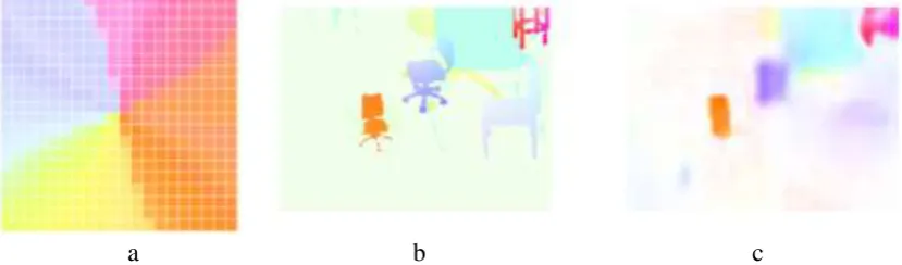
a b c

Variational Auto-encoder

To have a visualization of the latent manifold that generates the optical flow filed, we scan the latent plane, sampling latent points at regular intervals, and generating the corresponding optical flow field for each of these points. The results are demonstrated in Figure 3a. The decoded optical flow fields indicate the motion of the correspondence latent variable. The figure is somehow different from a flow color coding map. However, it is clear that there is a mapping relation between the latent variable and the optical flow. (There are lattice in the figure due to the input patch size is too small.) The variational take a ground optical flow ground truth as input, and reconstruct it. A reconstruction result is shown in Figure 3b, c. The motion information and the structure information is extracted by the encoder while the texture is loss.

Comparison with the State-of-the-Art

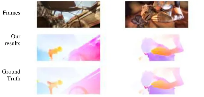
Figure 4 shows examples of our results on MPI-Sintel dataset. The average endpoint error on Flying Chairs and MPI-Sintel datasets are reported in Table 2.

Frames

Our results

Ground Truth

Figure 4. Examples on MPI-Sintel dataset. Table 2. Comparison with the state-of-the-art methods.

Method Flying Chairs MPI-Sintel

Epic Flow [16] 2.94 6.29

FlowNetS+v [13] 2.86 7.67

FlowNetS+ft+v 3.03 7.22

PatchBatch [14] - 6.78

Ours 3.04 5.85

The worse result on Flying Chairs dataset than FlowNetS is expected, for extra loss used in training. Unless the network parameters converge at the global minimal, the endpoint error will not be better than the result of network which is trained by using endpoint error only. Nevertheless, on the MPI-Sintel, the proposed method demonstrates that the perceptual loss as pairwise potentials leads to better generalization ability. Notice that the results of our method have no posterior variational refinement.

Conclusion

Acknowledgments

This work was supported by Shenzhen STP (JCYJ20150331151358150).

References

[1] Kalal, Zdenek, Krystian Mikolajczyk, and Jiri Matas. "Tracking-learning-detection." IEEE transactions on pattern analysis and machine intelligence 34.7 (2012): 1409-1422.

[2] Guo, Kai, Prakash Ishwar, and Janusz Konrad. "Action recognition using sparse representation on covariance manifolds of optical flow." Advanced Video and Signal Based Surveillance (AVSS), 2010 Seventh IEEE International Conference on. IEEE, 2010.

[3] Liu, Shuaicheng, et al. "Steadyflow: Spatially smooth optical flow for video stabilization." Proceedings of the IEEE Conference on Computer Vision and Pattern Recognition. 2014.

[4] Mathieu, Michael, Camille Couprie, and Yann LeCun. "Deep multi-scale video prediction beyond mean square error." arXiv preprint arXiv: 1511. 05440 (2015).

[5] Horn, Berthold KP, and Brian G. Schunck. "Determining optical flow." Artificial intelligence 17.1-3 (1981): 185-203.

[6] Zach, Christopher, Thomas Pock, and Horst Bischof. "A duality based approach for realtime TV-L 1 optical flow." Joint Pattern Recognition Symposium. Springer Berlin Heidelberg, 2007.

[7] Chen, Qifeng, and Vladlen Koltun. "Full flow: Optical flow estimation by global optimization over regular grids." Proceedings of the IEEE Conference on Computer Vision and Pattern Recognition. 2016.

[8] Bailer, Christian, Bertram Taetz, and Didier Stricker. "Flow fields: Dense correspondence fields for highly accurate large displacement optical flow estimation." Proceedings of the IEEE International Conference on Computer Vision. 2015.

[9] Menze, Moritz, Christian Heipke, and Andreas Geiger. "Discrete optimization for optical flow." German Conference on Pattern Recognition. Springer International Publishing, 2015.

[10] Johnson, Justin, Alexandre Alahi, and Li Fei-Fei. "Perceptual losses for real-time style transfer and super-resolution." European Conference on Computer Vision. Springer International Publishing, 2016.

[11] Zheng, Shuai, et al. "Conditional random fields as recurrent neural networks." Proceedings of the IEEE International Conference on Computer Vision. 2015.

[12] Eigen, David, and Rob Fergus. "Predicting depth, surface normals and semantic labels with a common multi-scale convolutional architecture." Proceedings of the IEEE International Conference on Computer Vision. 2015.

[13] Dosovitskiy, Alexey, et al. "Flownet: Learning optical flow with convolutional networks." Proceedings of the IEEE International Conference on Computer Vision. 2015.

[14] Gadot, David, and Lior Wolf. "Patchbatch: a batch augmented loss for optical flow." Proceedings of the IEEE Conference on Computer Vision and Pattern Recognition. 2016.

[15] Schuster, Tal, Lior Wolf, and David Gadot. "Optical Flow Requires Multiple Strategies (but only one network)." arXiv preprint arXiv: 1611. 05607 (2016).

[17] Shi, Wenzhe, et al. "Real-Time Single Image and Video Super-Resolution Using an Efficient Sub-Pixel Convolutional Neural Network." Computer Vision and Pattern Recognition (2016): 1874-1883.

[18] Kingma, Diederik P., and Max Welling. "Auto-Encoding Variational Bayes." stat 1050 (2014):1.