Comparison of GA Based Algorithms: A Viewpoint of Learning Scheme

2017 2nd International Conference on Communications, Information Management and Network Security (CIMNS 2017) ISBN: 978-1-60595-498-1

Comparison of GA-Based Algorithms: A Viewpoint of Learning Scheme

Guo-sheng HAO

, Qiu-yi Shi, Gai-ge WANG, Zhao-jun ZHANG

and De-xuan ZOU

School of Computer Science & Technology, Jiangsu Normal University, Xuzhou, 221116, China

*Corresponding author

Keywords: Genetic algorithm, Learning mechanism, Evolutionary operators, Learning rules.

Abstract. Learning is at the core of intelligence. How does learning work in nature-inspired optimization algorithms? This paper tries to answer this question by analyzing the learning mechanisms in Genetic Algorithm (GA) based Algorithms (GAAs). First, we give a learning scheme, which includes four basic elements including learning subject, learning object, learning result and learning rules. Different GAA has different learning mechanisms. Each GAA generates new solutions by learning to explore/exploit promising sub-space. The learning mechanism of three kinds of GAA, including GA, evolutionary strategy and differential evolution, are studied. We study the learning mechanism from the viewpoint of evolutionary operators, including selection, crossover (or recombination) and mutation. This study enables us to get more insights of GAAs.

Introduction

For many decades, researchers have been developing ever more sophisticated nature-inspired metaheuristic algorithms (NIOAs)[1] for solving hard optimization problems. Among NIOAs, Genetic Algorithm (GA) [2] was firstly introduced. Since then, various other optimization algorithms have been proposed such as Evolutionary Programming (EP) [3], Evolutionary Strategy (ES) [4] (which are know as GA based algorithm, GAAs), and so on.

Different NIOAs are inspired by different natural phenomena and may have different learning strategies or mechanisms to update their population. Yang pointed out that PSO and HS were the cases of BA, and the links among different NIOAs is intensification and diversification [5]. But the details of the similarities were not studied. There are, of course, many learning methods or many ways to generate new solutions. Regardless of the specific ways, it is generally agreed that NIOAs utilize operators to carry out learning or generate new solutions. Almost all NIOAs can correspond to the flowchart shown in Figure 1 (a), where different NIOAs can be compared briefly from the viewpoint of new solution generation, which is the result of learning mechanism.

Learning Scheme in Nature-inspired Optimization Algorithm

The learning schema in NIOAs are studied by answering the five questions.

What is the Learning Scheme? We study it from 3 aspects: who learns, from whom to learn and how to learn, and we study it from 4 elements in the learning scheme: learning subject XS, learning

object XO, learning result Xnew, and learning rule denoted as function L(∙). Figure 1 (b) demonstrates

the maximum optimization case. The learning subjects are B and D; the learning objects are F, G and H; the learning results are A, C and E.

Based on these specifications, two kinds of learning: learning by oneself and learning from others, can be formulated. For the first case, there is , where could be a random or constant step for XS to exploit. For the second case, the learning scheme is .

By leaning, an solution incorporate the experience of both its own and its learning object(s) [6] and the promising solutions is expected to satisfy .

, , where t is the iteration number. In machine learning,

labeled data are one of the most important resources for learning, and they are also well known as the training data. As intelligent algorithms, NIOAs also make well use of the labeled data, and EHI act as this role.

How does the Learning Mechanism Works? The learning in NIOAs is embedded in the update of population, which can be considered as the learning process. We explain “how to learn” in Figure 1 (c), in which the search space is denoted as S. Both {XS} and {XO} are subset of IH(t). By learning, the

algorithms will determine the promising solutions {Xnew}. We also call the nature-inspired operators

as learning operators, which act as the role to explore or exploit new space.

Begin Initialize

Terminate?

End

Generate new solutions step 1

Generate new solutions step n

Evaluate fitness Y

N

...

Differences among OAs

(a) General flowchart of optimization algorithms.

(b) New solutions generation based on learning from others.

(c) New solutions generation based on evolution history information.

Figure 1. General flowchart and new solution generation.

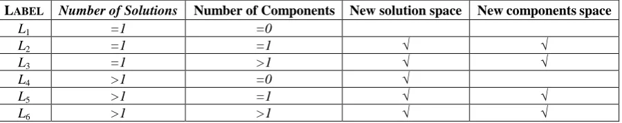
How Many Learning Type Are There? Almost all the learnings are carried out on two levels: solution level and components level. We classify learning operators according to the number of solutions, the number of components, new solution space and new components space. These learning operators are labeled as L1 to L6 that are shown in Table 1.

Table 1. Type of Learning Operators.

LABEL Number of Solutions Number of Components New solution space Newcomponentsspace

L1 =1 =0

L2 =1 =1 √ √

L3 =1 >1 √ √

L4 >1 =0 √

L5 >1 =1 √ √

L6 >1 >1 √ √

How to Measure Learning Results? If the learning result or results has the same peak with learning subjects (or learning objects , if applicable), we take it as granted that

the learning is exploitation. If the learning result or results has the different peak with learning subjects (or learning objects , if applicable), we take it as granted that the learning is exploration. The distance between the learning result and the learning subject cannot be a measurement for the learning result, especially for cheat problems. Similarly, other measurements that were mentioned in [8] such as difference, entropy, probability or ancestry are also not suitable for the learning result measurement.

Learning Mechanism in GA-based Nature-inspired Optimization Algorithms

Denote the number of dimension (variants) as d, and Di as the scope of i-th dimension. Variables in a

d-dimensional search space are presented as vectors.

Genetic Algorithms

Selection Operator. Selection is a learning operator, because it adjusts the structure of the population. The role of selection is to determine the learning objects from whom other solutions should learn in the successive learning operators. The learning subject and object in selection operator is . The expression of learning rule L(∙) is , . We can see that is the linear combination of solutions in P. From Figure 2, we can see that both in multi-modal and in single-modal case, the effect of selection is exploitation.

(a) Exploitation effect (b) Exploitation effect

Figure 2. An example of a 2-dimensional case of selection operator in GA.

Crossover Operator. The second learning step in GA is crossover operator, which is for sharing information among solutions that combines the good features of two or more parents, to create potentially better offspring. For example, two solutions and are selected as the crossover solutions and suppose that the crossover position is selected at k (1≤k<d). Then the learning subject and object are . Let

, , ,

, then the offspring of crossover are: , . We can label the result as: . The expression of learning rule L(∙) is

,

, where i=1, 2, …, d.

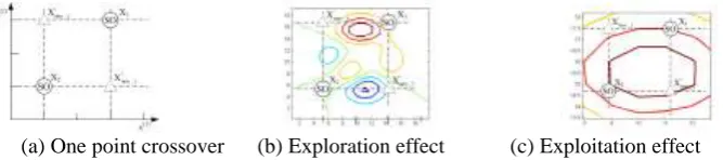
Crossover has the ability of exploration and exploitation. Figure 3 depicts the one-point crossover on the two-dimension variables case, from which we can see the exploration or exploitation.

(a) One point crossover (b) Exploration effect (c) Exploitation effect

Figure 3. An example of a 2-dimensional case for one crossover operator in GA.

Mutation Operator. Mutation operator randomly changes the values of some allele in the chromosome. Suppose that the mutation locus is k(1≤k≤d). Then the learning mechanism is

, , where . Let

, , ,

, then there is: . And the learning rule L(∙)

can be expressed as .

(a) Learning elements (b) Exploration effect (c) Exploitation effect (d) Learning with two-point

Figure 4. Space exploration/exploitation of one-point mutation for 2-dimensional case.

Evolutionary Strategy

Evolutionary strategy (ES) carry out competition between parent and offspring. ( ) ES has parent and offspring and is general in real application and (1+1) ES is the simplest style. There are also three learning steps in ES and they are selection, recombination and mutation.

Recombination Operator. There are mainly three kinds of recombination operators: discrete

recombination, intermediate recombination and weighted recombination. For all these three kinds of recombination operators, the learning subject and object are: , , where ρ is the number of parents, is consisted of solutions after selection. For the first case, the expression of learning rule L(∙) is:

. In intermediate recombination, a component will learn from all the parents, and the learning rule L(∙) takes a weighted average of all ρ parents as: . The space exploration of this recombination can be shown in Figure 10 (a)~(c) for ρ=2 and Figure 10 (d) for ρ=3 respectively, where the new solution is at the centre of the mass of learning subject and objects with mass value as 1. The third recombination is also a weighted recombination. For a maximum optimization, the learning rule L(∙) is . It is easy to know that the new

solution is nearer to the fit solutions than to other solutions, which is shown as in Figure 5 (e).

(a) Learning elements

(b) Exploration effect

(c) Exploration effect

(d) Learning with intermediate recombination

operator with three parents

(e) Learning with proportional recombination

Figure 5. An example of a 2-dimensional case for recombination operator in ES.

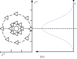
Mutation Operator. The mutation operator introduces variations by adding perturbation to a solution. For multi variants, the perturbation can be multivariate normal distribution, , with zero mean and covariance matrix . The learning subject and object are: , . The expression of learning rule L(∙) is: . And there is: . By the perturbation, Xnew_3 can access any solutions in the search space as shown in Figure 6.

x(1)

x(2)

x

f(x)

Differential Evolution

Differential evolution (DE) employs mutation and crossover operations to produce a trial solution. Then a selection operation is used to choose solutions for the next generation.

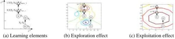
Mutation Operator. In DE, mutation is linear combination of solutions and the learning subject and object are: , , where Xj and Xk are randomly

chosen solutions from the population. The learning rule L(∙) is: , where is a scale factor within the range [0, 2], usually . is also referred to as perturbation to Xi.

There are many variants based on the basic learning rule, such as: 1) Leaning directly based on the best solution Xbest, instead of itself and the learning rule L(∙) is: ; 2)

Learning from more solutions instead of just two solutions as: , where Xj, Xk, Xm and Xn are randomly selected from the population. 3) Learning from the best

solution Xbest: . Similarly, based on Figure 7, we can

analyse the exploration and exploitation effect, we omit it here.

(a) Learning elements (b) Exploration effect (c) Exploitation effect

Figure 7. An example of a 2-dimensional case and the process for mutation operator in DE with .

Crossover Operator. The number of crossover-point in DE is equal to the number of components of a solution. The learning mechanism of crossover is

, , where pc is the crossover probability.

Selection Operator. In DE, selection is carried out after mutation and crossover and it is carried out based on competing between parents and offspring. The learning mechanism is:

,

Conclusion

This paper studies the learning mechanism in GAAs algorithms and give the nature of the evolutionary operators in GAAs. The comparison enables theory researchers to get the similarity and differences among GAAs, and also help the application researchers understand the integration of different GAAs together.

Acknowledgement

This work was partially supported by the National Science Foundation of China under Grants No. 61673196, 61503165, 61403174.

References

[1] K. Smith-Miles, and L. Lopes, “Measuring instance difficulty for combinatorial optimization problems,” Computers & Operations Research, 39(2012) 875-889.

[3] L. J. Fogel, A. J. Owens, and M. J. Walsh, Artificial intelligence through simulated evolution, New York: Wiley, 1966.

[4] I. Rechenberg, Evolution strategy: nature’s way of optimization, Optimization: Methods and Applications, Possibilities and Limitations, Lecture Notes in Engineering H. W. Bergmann, ed., pp. 106-126: Springer Berlin Heidelberg, 1989.

[5] X.-S. Yang, Nature-inspired metaheuristic algorithms: Luniver press, 2010.

[6] R. Eberhart, and Y. Shi, Comparison between genetic algorithms and particle swarm optimization, Evolutionary Programming VII, Lecture Notes in Computer Science V. W. Porto, N. Saravanan, D. Waagen and A. E. Eiben, eds., pp. 611-616: Springer Berlin Heidelberg, 1998.

[7] S. S. Sundar, S. Knobloch-Westerwick, and M. R. Hastall, News cues: information scent and cognitive heuristics, Journal of the American Society for Information Science and Technology, 58(2007) 366-378.