Analysis of stability for stochastic delay integro differential equations

R E S E A R C H

Open Access

Analysis of stability for stochastic delay

integro-differential equations

Yu Zhang

_{and Longsuo Li}

*_{Correspondence:} [email protected] 1_{Harbin University of Commerce} School of Economics, Harbin, China Full list of author information is available at the end of the article

Abstract

In this paper, we concern stability of numerical methods applied to stochastic delay integro-differential equations. For linear stochastic delay integro-differential equations, it is shown that the mean-square stability is derived by the split-step backward Euler method without any restriction on step-size, while the

Euler–Maruyama method could reproduce the mean-square stability under a step-size constraint. We also confirm the mean-square stability of the split-step backward Euler method for nonlinear stochastic delay integro-differential equations. The numerical experiments further verify the theoretical results.

Keywords: Stochastic delay integro-differential equations; Euler–Maruyama method; Split-step backward Euler method; Mean-square stability

1 Introduction

Stochastic delay integro-differential equations, as the mathematical model, widely apply in biology, physics, economics and finance [1, 2]. Because of the stochastic delay integro-differential equations themselves, it is not easy to obtain an explicit solution for these kinds of equations, so it is necessary to research the numerical methods for numerical solution of stochastic delay integro-differential equations [3, 4]. Stability is the basic and important property of numerical methods for stochastic systems.

There are few results on the numerical methods to stochastic delay integro-differential equations. Ding et al. [5] dealt with the stability of the semi-implicit Euler method for linear stochastic delay integro-differential equations. Rathinasamy and Balachandran [6] proved mean-square stability of the Milstein method for linear stochastic delay integro-differential equations with Markovian switching under suitable conditions on the inte-gral term. The condition under which the split-step backward Euler method was mean-square stable has been obtained by Tan and Wang [7, 8]. Rathinasamy and Balachan-dran [9] also analyzedT-stability of the split-step-θ-methods for linear stochastic delay integro-differential equations. Wu [10] investigated the mean-square stability for stochas-tic delay integro-differential equations by the strong balanced methods and the weak bal-anced methods with sufficiently small step-size. Numerical researches for stochastic delay integro-differential equations are not perfect enough. Therefore, it is extremely essential to develop the stability of the numerical methods to stochastic equations.

The paper is organized as follows. In Sect. 2 we will introduce related symbols and defini-tions. Some suitable conditions will be given to guarantee stability of the Euler–Maruyama

method for stochastic delay integro-differential equations in Sect. 3. In Sect. 4, the split-step backward Euler method will be used to prove general mean-square stability of nu-merical solutions. In Sect. 5, we will discuss stability of nonlinear stochastic delay integro-differential equations. Furthermore, numerical experiments are provided in Sect. 6.

2 Preliminaries

Throughout this paper, unless otherwise specified, let (,F,P) be a complete probability space with a filtration (Ft)t≥0, which satisfies the usual conditions (i.e., it is increasing and

right continuous whileF0contains allP-null sets). Let| · |be the Euclidean norm,W(t)

is Wiener process defined on the probability space, which be Ft-adapted and indepen-dent ofF0. Letτ> 0 andC([–τ, 0];R) denote the family of all continuousR-valued

func-tions on [–τ, 0],C([–τ, 0];Rd) denote the family of all continuous functionsξfrom [–τ, 0] to Rd_{,ξ is defined byξ=sup}

–τ≤t≤0|ξ(t)|. We assumeξ(t),t∈[–τ, 0] is the initial

function, which isF0-measurable and right continuous,Eξ2<∞. LetC_Fb₀([–τ, 0];R) be

the family of allF0-measurable boundedC([–τ, 0];R)-valued random variablesξ={ξ(θ) :

–τ≤θ≤0}.

As a matter of convenience, we first consider the following form of linear stochastic delay integro-differential equations:

⎧ ⎪ ⎨ ⎪ ⎩

dx(t) = [αx(t) +βx(t–τ) +γ_tt_–τx(s)ds]dt

+ [λx(t) +μx(t–τ) +η_tt_–τx(s)ds]dW(t), t≥0, x(t) =ξ(t), t∈[–τ, 0],

(1)

whereξ(t) is initial function, andξ(t)∈C([–τ, 0];R),α,β,γ,λ,μ,η∈R,W(t) is a standard one-dimensional Wiener process andτ is the delay term.

Under the above assumptions, Eq. (1) has a unique solution x(t). In order to analyze mean-square stability of two numerical methods, we introduce the following lemma [11].

Lemma 2.1 If

α+|β|+|γ|τ+1 2

|λ|+|μ|+|η|τ2< 0 (2)

the solution of Eq. (1)is said to be mean-square stable,that is,

lim t→∞E x(t)

2

= 0. (3)

3 Mean-square stability of the Euler–Maruyama method

Now, the Euler–Maruyama method applied to Eq. (1) one gets

Xn+1=Xn+ (αXn+βXn–m+γXn¯ )h+ (λXn+μXn–m+ηXn¯ )Wn, (4)

where ξ =X0, Xn is an approximation to the analytical solution x(tn),n which isFtn

paper will choose a composite trapezoidal rule as the tool of the disperse integral to solve this case. We have

¯ Xn=h

2Xn–m+h m–1

k=1

Xn–k+ h 2Xn.

Definition 3.1 If there exists ah0> 0, for every step-sizeh∈(0,h0] withh=_mτ, such that

the numerical approximation{Xn}produced by the Euler–Maruyama method satisfies

lim n→∞E|Xn|

2_{= 0 (5)}

then the numerical method applied to Eq. (1) is said to be mean-square stable.

Theorem 3.1 Under the condition(2),let h0=max{h1,h2},for step-size h∈(0,h0],we have

lim n→∞E|Xn|

2_{= 0}

then the Euler–Maruyama method applied to Eq. (1)is mean-square stable,where

h1= –

2α+ 2|β|+ 2|γ|τ+ (|λ|+|μ|+|η|τ)2

(|α|+|β|+|γ|τ)2 ,

h2=min

–1

α, –

2α+ 2|β|+ 2|γ|τ+ (|λ|+|μ|+|η|τ)2

(α+|β|+|γ|τ)2

.

Proof From Eq. (4), we obtain

Xn+1= (1 +αh+ηWn)Xn+ (βh+μWn)Xn–m

+ (γh+ηWn)Xn¯ . (6)

Squaring both sides of Eq. (6), we have

X_n2₊₁= (1 +αh+ηWn)2X2_n+ (βh+μWn)2X_n2_–m+ (γh

+ηWn)2X¯n2+ 2(1 +αh+ηWn)(βh+μWn)XnXn–m

+ 2(1 +αh+ηWn)(γh+ηWn)XnXn¯

+ 2(βh+μWn)(γh+ηWn)Xn–mXn¯

=1 +α2h2+λ2W_n2+ 2αh+ 2λWn+ 2αλhWnX_n2

+β2h2+ 2βμhWn+μ2W_n2X_n2_–m+γ2h2

+ 2γ ηhWn+η2Wn2

_¯

X_n2+ 2βh(1 +αh+ηWn)

+μWn(1 +αh+ηWn)XnXn–m+ 2

γh(1 +αh+ηWn)

+ηWn(1 +αh+ηWn)XnXn¯

It follows from 2ab≤ |ab|(x2_+y2_{), wherea,b∈R,τ=mh, that}

2Xn–mXn¯ = 2Xn–m

h

2Xn–m+h m–1

k=1

Xn–k+ h 2Xn

=hX_n2_–m+ 2hXn–m m–1

k=1

Xn–k+hXnXn–m

≤hX_n2_–m+h(m– 1)X_n2_–m+h m–1

k=1

X_n2_–k+h 2

X_n2+X_n2_–m

≤τX_n2_–m+h 2X

2

n–m+h m–1

k=1

X_n2_–k+h 2X

2

n. (7)

According to the inequality (a1+a2+· · ·+an)2≤n(a21+a22+· · ·+a2n),

¯ X_n2=h2

1 2Xn–m+

m–1

k=1

Xn–k+ 1 2Xn

2

≤h2

1 4X

2

n–m+ (m– 1) m–1

k=1

X_n2_–k+1 4X 2 n+ 1 2

(m– 1)X_n2_–m

+ m–1

k=1

X_n2_–k

+1 2

X2_n+X_n2_–m+1 2

(m– 1)X2_n+ m–1

k=1

X_n2_–k

≤τ h 2X 2

n–m+h m–1

k=1

X2_n–k+h 2X

2

n

. (8)

In a similar way

2XnXn¯ =τX_n2+h 2X

2

n–m+h m–1

k=1

X2_n–k+h 2X

2

n. (9)

We note thatE(Wn) = 0,E[(Wn)2_{] =h, andXn,Xn}

–1, . . . ,Xn–mareFtn-measurable.

Sub-stituting (7), (8), (9) into the above equation and taking expectations,

EX_n2₊₁≤1 +α2h2+λ2h+ 2αhEX_n2+β2h2+μ2hEX_n2_–m

+γ2h2+η2hτE

h 2X

2

n–m+h m–1

k=1

X_n2_–k+h 2X

2

n

+ (1 +αh)βh +|λμ|hEX_n2+EX_n2_–m

+ (1 +αh)γh +|λη|hE

τX_n2+h 2X

2

n–m

+h m–1

k=1

X2_n–k+h 2X

2

n

+|βγ|h2+|μη|h

×E

τX_n2_–m+h 2X

2

n–m+h m–1

k=1

X_n2_–k+h 2X

2

n

LetYn=E|X2

n|, we have

Yn+1≤PYn+QYn–m+R max n–m≤i≤n(Yi), where

P= 1 +α2h2+λ2h+ 2αh+ (1 +αh)βh +|λμ|h+|λη|τh

+ (1 +αh)γ τh ,

Q=β2h2+μ2h+ (1 +αh)βh +|λμ|h+|βγ|τh2+|μη|τh,

R=γ2h2+η2hτ2+ (1 +αh)γ τh +|λη|τh+|βγ|τh2+|μη|τh.

So

Yn+1≤(P+Q+R)max

Yn,Yn–m, max n–m≤i≤n(Yi)

.

It is clear thatYn→0 (n→ ∞) ifP+Q+R< 1, namely

1 +α2h2+λ2h+ 2αh+ 2 (1 +αh)βh + 2|λμ|h+ 2|λη|τh+β2h2+μ2h

+ 2 (1 +αh)γ τh + 2|βγ|τh2+ 2|μη|τh+γ2h2+η2h< 1.

Hence let

h1= –

2α+ 2|β|+ 2|γ|τ+ (|λ|+|μ|+|η|τ)2

(|α|+|β|+|γ|τ)2 ,

h2=min

–1

α, –

2α+ 2|β|+ 2|γ|τ+ (|λ|+|μ|+|η|τ)2

(α+|β|+|γ|τ)2

.

By the condition (2), we know thath1> 0,h2> 0. Ifh0∈(0,h1), we have

α2+ 2|αβ|+ 2|αγ|τ+β2+ 2|βγ|τ+γ2τ2h2

+2α+ 2|β|+ 2|γ|τ+|λ|+|μ|+|η|τ2h< 0.

On the other side, we address the case 1 +αh> 0. Ifh0∈(0,h2), we get

α2+ 2α|β|+ 2α|γ|τ+β2+ 2|βγ|τ+γ2τ2h2

+2α+ 2|β|+ 2|γ|τ+|λ|+|μ|+|η|τ2h< 0.

Leth0∈max{h1,h2}; whenh∈(0,h0],P+Q+R< 1 always holds, then

lim

n→∞Yn=nlim→∞E|Xn|

2_{= 0}

then the Euler–Maruyama method applied to Eq. (1) is mean-square stable. The theorem

4 General mean-square stability of the split-step backward Euler method

Using the split-step backward Euler method applied to Eq. (1), we construct the numerical scheme as follows:

X_n∗=Xn+ (αX_n∗+βXn–m+γXn¯ )h, Xn+1=X∗n+ (λXn∗+μXn–m+ηXn¯ )Wn;

(10)

the relevant definitions are in Sect. 3, if 1 –αh= 0, we can get the sequences{X∗_n,n≥0} and{Xn,n≥1}via (10), when givenXn=ξ(nh) forn∈ {–m, –m+ 1, . . . , 0}.

Definition 4.1 For every step-sizeh= τ

m, if any application of the split-step backward Euler method to Eq. (1) generates a numerical approximation{Xn}that satisfies

lim n→∞E|Xn|

2_{= 0 (11)}

then the numerical method applied to Eq. (1) is said to be general mean-square stable.

Theorem 4.1 Under the condition(2),assume1 –αh= 0,the split-step backward Euler method applied to Eq. (1)is generally mean-square stable.

Proof Assume 1 –αh= 0 and implyingα< 0; we can see from (10) that

Xn+1=

1 +λWn

1 –αh (Xn+βhXn–m+γhXn¯ ) + (μXn–m+ηXn¯ )Wn. (12)

Squaring both sides of Eq. (12),

X_n2₊₁=

1 +λWn 1 –αh

2

X_n2+β2h2X_n2_–m+γ2h2X¯_n2+ 2βhXnXn–m+ 2γhXnX¯n

+ 2βγh2Xn–mXn¯

+μ2X_n2_–m+η2X¯_n2+ 2μηXn–mXn¯

W_n2

+ 21 +λWn

1 –αh (Xn+βhXn–m+γhX¯n)(μXn–m+ηX¯n)Wn.

According to 2abxy≤ |ab|(x2_+y2_{) andE(Wn) = 0,E[(Wn)}2_{] =h, substituting (7), (8),}

(9) into the above equation and taking expectations

EX_n2₊₁≤ 1 +λ

2_h

(1 –αh)2

EX_n2+β2h2EX_n2_–m+γ2h2τE

h 2X

2

n–m

+h m–1

k=1

X2_n–k+h 2X

2

n

+|β|hEX2_n+EX_n2_–m

+|γ|hE

τXn+h 2X

2

n–m+h m–1

k=1

X_n2_–k+h 2X

2

n

+|βγ|h2E

τXn–m+ h 2X

2

n–m+h m–1

k=1

X_n2_–k+h 2X

2

n

+μ2hEX_n2_–m+η2τhE

h 2X

2

n–m+h m–1

k=1

X_n2_–k+h 2X

2

n

+|μη|hE

τXn–m+ h 2X

2

n–m+h m–1

k=1

X_n2_–k+h 2X

2

n

+ |λμ|h 1 –αh

EX_n2+EX_n2_–m+2|βλμ|h

2

1 –αh EX

2

n–m

+|γ λμ|h

2

1 –αh E

τXn–m+ h 2X

2

n–m+h m–1

k=1

X_n2_–k+h 2X

2

n

+ |λη|h 1 –αhE

τXn+ h 2X

2

n–m+h m–1

k=1

X_n2_–k+h 2X

2

n

+|βλη|h

2

1 –αh E

τXn–m+ h 2X

2

n–m+h m–1

k=1

X_n2_–k+h 2X

2

n

+2|γ λη|h

2

1 –αh τE

h 2X

2

n–m+h m–1

k=1

X2_n–k+h 2X 2 n , in particular

EX_n2₊₁≤PEX_n2+QEX_n2_–m+R max n–m≤i≤nE

X_i2,

where

P= 1 +λ

2_h

(1 –αh)2

1 +|β|h+|γ|hτ+|λη|hτ 1 –αh +

|λμ|h 1 –αh,

Q= 1 +λ

2_h

(1 –αh)2

β2h2+|β|h+|βγ|τh2+μ2h+|μη|τh

+ |λμ|h 1 –αh+

|βλη|τh2

1 –αh +

|γ λμ|τh2

1 –αh +

2|βλμ|h2

1 –αh ,

R= 1 +λ

2_h

(1 –αh)2

γ2h2τ2+|γ|τh+|βγ|τh2+η2τ2h+|μη|τh

+|γ λμ|τh

2

1 –αh + |λη|τh 1 –αh+

|βλη|τh2

1 –αh +

2|γ λη|h2

1 –αh τ

2_.

LetYn=E|Xn2|, the above inequality turns into

Yn+1≤(P+Q+R)max

Yn,Yn–m, max n–m≤i≤nYi

.

We conclude thatYn→0 (n→ ∞), ifP+Q+R< 1, that is,

1 +λ2h (1 –αh)2

1 +|β|h+ 2|γ|hτ2+2|λμ|h 1 –αh +

2|λη|τh 1 –αh +

2|βλμ|h2 1 –αh

+2|γ λμ|τh

2

1 –αh +

2|βλη|τh2

1 –αh +

2|γ λη|τ2h2

1 –αh +

Hence, we have

|βλ|+|γ λ|τ–α|μ|+|η|τ2h2+|β|+|γ|τ2–α2

+2|λ|+ 2|μ|+ 2|η|τ|βλ|+|γ λ|τ–α|μ|+|η|τh

+ 2α+ 2|β|+ 2|γ|τ+|λ|+|μ|+|η|τ2< 0.

Let

F(h) =Ah2+Bh+ 2α+ 2|β|+ 2|γ|τ+|λ|+|μ|+|η|τ2,

where

A=|βλ|+|γ λ|τ–α|μ|+|η|τ2,

B=|β|+|γ|τ2–α2+2|λ|+ 2|μ|+ 2|η|τ|βλ|+|γ λ|τ–α|μ|+|η|τ,

=|β|+|γ|τ2–α2+2|λ|+ 2|μ|+ 2|η|τ|βλ|+|γ λ|τ–|μ|+|η|τ2

– 4|βλ|+|γ λ|τ–α|μ|+|η|τ22α+ 2|β|+ 2|γ|τ+|λ|+|μ|+|η|τ2.

It is easy to seeA> 0, Because of the nature of a quadratic function, we can see thatF(h) < 0 holds for any 0 <h< 1, when –B+

√

2A ≥1, and the split-step backward method Euler is general mean-square stable. This proves the theorem.

5 Mean-square stability of the split-step backward Euler method for nonlinear stochastic systems

In this section, we will discuss the mean-square stability of the split-step backward Eu-ler method for nonlinear stochastic delay integro-differential equations. Considering the following nonlinear stochastic equation:

⎧ ⎪ ⎨ ⎪ ⎩

dx(t) =f(x(t),x(t–τ),_tt_–τx(s)ds)dt

+g(x(t),x(t–τ),_tt_–τx(s)ds)dW(t), t≥0, x(t) =ξ(t), t∈[–τ, 0],

(13)

f :Rd_×Rd_×Rd_→Rd_,g:Rd_×Rd_×Rd_→Rd×m_{,ξ(t)∈C([–τ, 0];R}d_{),W(t) is anm} -dimensional Wiener process andτis a delay term. Iffandgare sufficiently smooth and sat-isfy the Lipschitz condition and the linear growth condition, Eq. (13) has a unique strong solutionx(t),t∈[–τ,∞) andx(t) is a measurable, sample-continuous and Ft adapted process [12, 13].

The split-step backward Euler method applied to Eq. (13) yields

X_n∗=Xn+f(Xn∗,Xn–m,X¯n)h, Xn+1=X∗n+g(Xn∗,Xn–m,X¯n)Wn;

(14)

Xn,X_n∗,Xn¯ ,h,Wnare defined in Sects. 3 and 4.

Lemma 5.1([14]) If there exist constant a1,a2,a3,b1,b2,b3,for all x,u,v∈Rd,we have

f(x,u,v) –f(x, 0, 0) ≤a2|u|+a3|v|, (16)

g(x,u,v) 2≤b1|x|2+b2|u|2+b3|v|2. (17)

Theorem 5.1 Suppose that Lemma5.1holds and let

–a1+a2+a3τ+

1 2

b1+b2+b3τ2

< 0. (18)

If there exists a h0> 0,for every step-size h∈(0,h0],we have

lim n→∞E|Xn|

2_{= 0.}

Then the numerical solution of Eq. (13)is mean-square stable,where

h0= –

–2a1+ 2a2+ 2a3τ+ (b1+b2+b3τ2)

b1(a2+a3τ) + (b2+b3τ2)(2a1–a2–a3τ)

.

Proof From the second equation of (14), we obtain

|Xn+1|2= Xn∗

2

+ gX_n∗,Xn–m,X¯n

2

W_n2+ 2X_n∗,gX_n∗,Xn–m,X¯n

Wn

.

Note thatE(Wn) = 0,E[(Wn)2_{] =h, andXn,Xn}

–m,X¯ areFtn-measurable, hence

EX_n∗,gX_n∗,Xn–m,Xn¯

Wn= 0,

E gX_n∗,Xn–m,Xn¯ 2Wn2= g

X_n∗,Xn–m,Xn¯ 2h.

Combining condition (17) and taking expectations on both sides of the above equation,

E|Xn+1|2≤E Xn∗

2

+b1E Xn∗

2

+b2E|Xn–m|2+b3E| ¯Xn|2

h

≤(1 +b1h)E Xn∗

2

+b2hE|Xn–m|2+b3hE| ¯Xn|2.

Next, we should derive theE|X_n∗|2by the first equation of (14),

X_n∗–fX∗_n,Xn–m,Xn¯

h=Xn. (19)

Squaring both sides of Eq. (19), one gets

X∗_n 2≤ |Xn|2+ 2hX∗_nfX∗_n,Xn–m,Xn¯

. (20)

Through the conditions (15), (16), we have

2X_n∗,fX∗_n,Xn–m,Xn¯

= 2X_n∗,fX_n∗, 0, 0+ 2X_n∗,fX∗_n,Xn–m,Xn¯

–fX_n∗, 0, 0 ≤–2a1 Xn∗

2

+a2 Xn∗

2

+|Xn–m|2

It is easily to see that forX_n∗Xn¯ from Sect. 3

2X_n∗Xn¯ =τX∗_n+h 2X

2

n–m+h m–1

k=1

X_n2_–k+h 2X

2

n.

Substituting these into Eq. (20) and taking expectations

E X_n∗ 2≤E|Xn|2– 2a1hE X∗n

2

+a2hE Xn∗

2

+|Xn–m|2

+a3h

τX_n∗+h 2X

2

n–m+h m–1

k=1

X_n2_–k+h 2X

2

n

≤(–2a1h+a2h+a3hτ)E Xn∗

2

+E|Xn|2+a2hE|Xn–m|2

+a3hτ max

n–m≤i≤nE|Xi|

2_.

In particular

E X_n∗ 2≤ 1

1 + 2a1h–a2h–a3hτ

E|Xn|2+ a2h

1 + 2a1h–a2h–a3hτ

E|Xn–m|2

+ a3hτ 1 + 2a1h–a2h–a3hτ

max n–m≤i≤nE|Xi|

2_.

Hence

E|Xn+1|2≤(1 +b1h)E Xn∗

2

+b2hE|Xn–m|2+b3hE| ¯Xn|2

≤ 1 +b1h

1 + 2a1h–a2h–a3hτ

E|Xn|2+

a2h(1 +b1h)

1 + 2a1h–a2h–a3hτ

+b2h

×E|Xn–m|2+

a3hτ(1 +b1h)

1 + 2a1h–a2h–a3hτ

+b3hτ2

max n–m≤i≤nE|Xi|

2_.

We can write

E|Xn+1|2≤PE|Xn|2+QE|Xn–m|2+R max n–m≤i≤nE|Xi|

2_,

where

P= 1 +b1h 1 + 2a1h–a2h–a3hτ

, Q= a2h(1 +b1h) 1 + 2a1h–a2h–a3hτ

+b2h,

R= a3hτ(1 +b1h) 1 + 2a1h–a2h–a3hτ

+b3hτ2.

So

E|Xn+1|2≤(P+Q+R)

E|Xn|2,E|Xn–m|2, max n–m≤i≤nE|Xi|

IfP+Q+R< 1, it is easily to see thatE|Xn|2_{→0 whenn→ ∞. By the condition (18), we}

have

b1(a2+a3τ) +

b2+b3τ2

(2a1–a2–a3τ)

h2+–2a1+ 2a2+ 2a3τ

+b1+b2+b3τ2

h< 0.

Namely

a2h+a3hτ+b1h+a2b1h2+a3b1τh2+b3hτ2+b3τ2(2a1–a2–a3τ)h2

+b2h+b2(2a1–a2–a3τ)h2– 2a1h+a2h+a3hτ< 0.

Therefore, for every step-sizeh∈(0,h0],limn→∞E|Xn|2= 0 holds, the split-step backward

Euler method for nonlinear stochastic equations is mean-square stable. The proof is

com-plete.

6 Numerical experiments

In this section, we will discuss the example to verify the theoretical results, considering the following testified equation:

⎧ ⎪ ⎨ ⎪ ⎩

dx(t) = [αx(t) +βx(t– 1) +γ_tt_–1x(s)ds]dt

+ [λx(t) +μx(t– 1) +η_tt_–1x(s)ds]dW(t), t≥0, x(t) =ξ(t), t∈[–1, 0].

(21)

Taking the parametersα= –10,β= 2,γ = 1,λ= 0.5,μ= 0.2,η= 0.5, the condition (2) is satisfied.

Case 1. We can easily see that h1= 12.56₁₆₉ , h2=min{₁₀1,12.56₄₉ }. By Theorem 3.1, h0=

max{h1,h2}=₁₀1. When the step-sizeh∈(0,₁₀1], the Euler–Maruyama method applied to

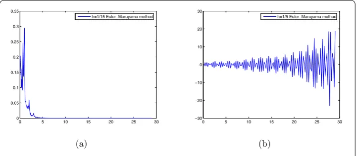
Eq. (21) is mean-square stable. However, the Euler–Maruyama method is unstable when the step-sizeh=1₅>₁₀1, which is shown in Fig. 1(a) and (b).

Case 2.We can knowA= [(|βλ|+|γ λ|τ) –α(|μ|+|η|τ)]2_{> 0,}–B+√

2A ≈1.13 > 1, and the conditions satisfy Theorem 4.1. Hence for any 0 <h< 1, the split-step backward method

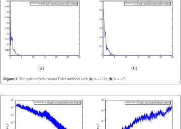
Figure 2The split-step backward Euler method with (a)h= 1/15; (b)h= 1/5

Figure 3The split-step backward Euler method with (a)h= 1/100; (b)h= 1/10

Euler has general square stability. From Fig. 2, it is easy to confirm general mean-square stability of a numerical solution under the same step-size as Case 1. The results indicate that the split-step backward Euler method achieves superiority over the Euler– Maruyama method in terms of mean-square stability.

Case 3.We will address the following nonlinear stochastic delay integro-differential equation:

⎧ ⎪ ⎨ ⎪ ⎩

dx(t) = [–80x(t) + 10x(t– 1) + 10_tt_–1x(s)ds]dt

+ [0.4x(t) + 0.4x(t– 1) + 4_tt_–1x(s)ds]dW(t), t≥0, x(t) = 1, t∈[–1, 0].

(22)

It is easy to ascertain that Eq. (22) satisfies the conditions of Lemma 5.1. So

a1= 80, a2= 10, a3= 10, b1= 2, b2= 2, b3= 20, τ = 1.

Therefore

–a1+a2+a3τ+

1 2

b1+b2+b3τ2

We should calculate the step-sizeh0≈0.03 from Theorem 5.1, the data used in all figures

are plotted by 200 trajectories. It is proved that the split-step backward Euler method has mean-square stability whenh= 0.01, whilehdissatisfied (0,h0], that is,h= 0.1 >h0, the

split-step backward Euler method is unstable. This is shown in Fig. 3.

7 Conclusion

In this paper, we investigate the mean-square stability and general mean-square stability of two numerical methods for a class of linear stochastic delay equations. By comparison, we know that the split-step backward Euler method achieves superiority over the Euler– Maruyama method in terms of mean-square stability. The mean-square stability of nu-merical method for nonlinear stochastic delay integro-differential equations is eventually confirmed by us.

Acknowledgements

The authors would like to thank the reviewers for their very valuable comments and helpful suggestions which improved the paper significantly.

Funding

No funding was received. Yu Zhang and his teacher professor Longsuo Li finished the manuscript together.

Competing interests

The authors declare that they have no competing interests.

Authors’ contributions

All authors read and approved the final manuscript.

Author details

1_{Harbin University of Commerce School of Economics, Harbin, China.}2_{Department of Mathematics, Harbin Institute of} Technology, Harbin, China.

Publisher’s Note

Springer Nature remains neutral with regard to jurisdictional claims in published maps and institutional affiliations.

Received: 25 December 2017 Accepted: 25 April 2018

References

1. Appleby, A.D., Riedle, Z.: Almost sure asymptotic stability of stochastic Volterra integro-differential equations with fading perturbations. Stoch. Anal. Appl.24(4), 813–826 (2006)

2. Mao, X.R., Riedle, F.: Mean square stability of stochastic Volterra integro-differential equations. Syst. Control Lett.55(4), 459–465 (2006)

3. Mokkedem, F.Z., Fu, X.L.: Approximate controllability of semi-linear neutral integro-differential systems with finite delay. Appl. Math. Comput.42(2), 205–215 (2014)

4. Yu, Z.H., Liu, M.Z.: Almost surely asymptotic stability of numerical solutions for neutral stochastic delay differential equations. Discrete Dyn. Nat. Soc.45(2), 1–11 (2011)

5. Ding, X.H., Wu, K.N., Liu, M.Z.: Convergence and stability of the semi-implicit Euler method for linear stochastic delay integro-differential equations. Int. J. Comput. Math.83(10), 753–763 (2006)

6. Rathinas, A., Balachandran, K.: Mean-square stability of Milstein method for linear hybrid stochastic delay integro-differential equations. Nonlinear Anal. Hybrid Syst.2(4), 1256–1263 (2008)

7. Tan, J., Wang, H.: Convergence and stability of the split-step backward Euler method for linear stochastic delay integro-differential equations. Math. Comput. Model.51(5), 504–515 (2010)

8. Jiang, F., Shen, Y., Liao, X.X.: A note on stability of the split-step backward Euler method for linear stochastic delay integro-differential equations. J. Syst. Sci. Complex.25(5), 873–879 (2012)

9. Rathinasamy, A., Balachandran, K.:T-stability of the split-stepθ-methods for linear stochastic delay integro-differential equations. Nonlinear Anal. Hybrid Syst.5(6), 639–646 (2011)

10. Wu, Q., Hu, L., Zhang, Z.J.: Convergence and stability of balanced methods for stochastic delay integro-differential equations. Appl. Math. Comput.237(7), 446–460 (2014)

11. Hu, P., Huang, C.M.: Stability of stochasticθ-methods for stochastic delay integro-differential equations. Int. J. Comput. Math.88(7), 1417–1429 (2011)

12. Mao, X.R.: Stochastic Differential Equation and Application. Horwood, Chischester (1997)

13. Li, Q.Y., Gan, S.Q., Zhang, H.M.: Mean-square exponential stability of an improved split-step backward Euler method for stochastic delay integro-differential equations. J. Numer. Methods Comput. Appl.34(2), 241–248 (2013) 14. Li, Q.Y., Gan, S.Q.: Mean-square exponential stability of stochasticθmethods for nonlinear stochastic delay