Soft Image Segmentation Based on the Mixture of Gaussians and the Phase Transition Theory

(1)

http://dx.doi.org/10.4236/am.2014.518275

How to cite this paper: Barcelos, C.A.Z., Chen, Y.M. and Chen, F.H. (2014) Soft Image Segmentation Based on the Mixture of Gaussians and the Phase-Transition Theory. Applied Mathematics, 5, 2888-2898.

http://dx.doi.org/10.4236/am.2014.518275

Soft Image Segmentation Based on the

Mixture of Gaussians and the

Phase-Transition Theory

Celia A. Z. Barcelos1*, Yunmei Chen2, Fuhua Chen3

1_{Faculty of Mathematics, Federal University of Uberlândia, Uberlândia, MG, Brazil} 2_{Department of Mathematics, University of Florida, Gainesville, FL, USA}

3_{Department of Natural Science & Mathematics, West Liberty University, West Liberty, WV, USA}

Email: *_{[email protected]}_,_{[email protected]}_,_{[email protected]}

Received 24 July 2014; revised 28 August 2014; accepted 15 September 2014

This work is licensed under the Creative Commons Attribution International License (CC BY). http://creativecommons.org/licenses/by/4.0/

Abstract

In this paper, we propose a new soft multi-phase segmentation model where it is assumed that the pixel intensities are distributed as a Gaussian mixture. The model is formulated as a minimization problem through the use of the maximum likelihood estimator and phase-transition theory. The mixture coefficients, which are estimated using a spatially varying mean and variance procedure, are used for image segmentation. The experimental results indicate the effectiveness of the me-thod.

Keywords

Image Segmentation, Variational Model, Gaussian Mixture

1. Introduction

Image segmentation is one of the most extensively studied problems in image processing and computer vision. Many different approaches have been proposed for the partitioning of images based on a variety of criteria including brightness (intensity), color, or texture. In general the partitioning of an image or detection of edges is under the assumption that an image consists of several patterns, and each point on the image domain belongs exclusively to only one pattern. Finding boundaries separating the different patterns in this sense is called a hard segmentation. Different to hard segmentation, soft segmentation assumes that each point may belong to more than one pattern. The goal of soft segmentation is to find all the probabilities that each pixel can belong to each

(2)

pattern. This probability is also called membership (or ownership) in the literature.

One of the most extensively studied approaches for hard segmentation is the variational method. Many effective variational models have been developed, for instance, the Mumford-Shah model [1], geodesic active contour [2], geodesic active region [3], and region competition [4]. Level set technique [5] has been proven to be powerful in the implementation of variational models. In two-phase segmentation the composition of the Heaviside function with the level set function is used to represent the regions of the object and background. In [6] [7], the authors extended the level set method to multiphase segmentation by using multiple level set functions, while in [8] [9], the authors proposed another means to extend the level set method by using multiple layers for each level set function. Through the act of carefully choosing the initial values, these methods can work very well. However, the non-convexity of the energy functional in the level set formulation is an inherent drawback of the level set method. As a result, many level set based variational segmentation models are sensitive to initial values and may converge to an undesirable local minimum. This problem is more difficult to deal with for multiphase segmentation.

To overcome the non-convexity problem mentioned above, one approach is to replace the composition of the heaviside function with the level set function in level set formulation by use of a weight/membership function. Through the implementation of this modification the energy is convex with respect to the membership function. For example, Chan et al. [10] and Bresson et al. [11] stated certain non-convex minimization problems for image segmentation and denosing as equivalent convex minimization problems by using membership functions to replace characteristic functions. These new models allow for the finding of global minimizers via standard convex minimization schemes. In particular in [11] efficient and fast numerical schemes to globally minimize the variational segmentation models were proposed. These algorithms are based on a dual formulation of the TV norm proposed and developed in [12]-[16].

Soft segmentation is also motivated by its applications to real world problems. In medical imaging, due to limited spacial resolution of the equipment, not all the voxels in a segmented region contain the same tissue type, especially near the boundary of two subregions. A typical example is the partial volume effect in MRI brain image segmentation. Instead of labeling each image voxel with a unique tissue type [17], partial volume segmentation aims at estimating the percentage of each voxel belonging to each tissue, which can be viewed as the probability of the voxel belonging to the tissue. Since soft segmentation allows each pixel to belong to several patterns with certain probabilities, it provides a more flexible mechanism, and thereby keeps more options available for post-processing steps.

There have been many soft segmentation methods. Mory and Ardon extended the original region competition model [4] to a fuzzy region competition method [18] [19]. The technique generalizes some existing supervised and unsupervised region-based model. The proposed functional is convex, which guarantees the global solution in the supervised case. Unfortunately, this method only applies to two-phase segmentation and is difficult to extend to multiphase segmentation. The fuzzy C-mean (FCM) [17] [20] [21] is a method developed for pattern classification and recognition. Hence it is also applicable to image segmentation. The standard FCM model partitions a data set

{ }

xk Nk=₁⊂Rd into M clusters by the following objective function [22] [23]

2

FCM 2

1 1

N M

ik i k i k

J u x v

= =

=

∑∑

− (1)

where uik is the membership value of datum xi for class k with 1 1 M

ik k=u =

∑

, and vk stands for the

cluster centers. The original FCM method is very sensitive to noise. An adaptive fuzzy c-means (AFCM) was proposed by Pham et al. [21], where the constant cluster centers used in the FCM model are substituted by spatially varying functions. The energy functional can be written as

( )

2

AFCM 2

1 1

N M

ik i i k i k

J u x m v G m

= =

=

∑∑

− + (2)

where m is the bias field and G m

( )

is the regularization term for the bias field m. AFCM is more robust to noise than the standard FCM. The soft segmentation model developed in [17] used a different similarity measure to that in [21]. Their objective functional reads as

(

)

(

)

(

)

AFCM

1 1 1 1

1 1

k

N M N M

ik i k ik r k

i k k i k r N

J u K x v u K x v

N

σ α σ

= = = = ∈

(3)

where

( )

, exp 2 ,

x y

K_σ x y

σ

 − − 

= _ _

  (4)

k

N stands for the set of neighbors falling into a window around x_k, and N_k is its cardinality. The parameter α in the second term controls the effect of the penalty.

Another class of soft segmentation is based on stochastic approaches. It considers that pixel intensities are independent samples from one or several distributions. The likelihood functions have been widely used in soft segmentation. In [24] the maximum-likelihood (ML) is used to find the optimal parameters in the joint pdf such that the likelihood function is maximized. An expectation-maximization (EM) algorithm is used to solve the problem when we are dealing with incomplete data. However, simply using likelihood to model an image is not enough since it ignored the prior knowledge of an image. In [25] the authors proposed an adaptive segmentation method that uses the knowledge of tissue properties and intensity inhomogeneities to correct and segment MR images. The EM algorithm was used to iteratively estimate the posterior tissue class probabilities when the bias field is known, and having a maximum a posteriori principle (MAP) estimator of the bias field, when tissue class probabilities are known.

In [20], a segmentation framework based on the MAP principle was proposed for partial volume (PV) segmentation of magnetic resonance brain images. A mixture of the probability density functions is considered to address the PV effect. A Markov Random Field (MRF) model is used to define the prior distribution of the mixture coefficient field imposing a smoothness on the mixture coefficients (ownerships). The fuzzy c-means model is extended to define the likelihood function of the observed image.

The phase transition theory in material sciences and fluid mechanics have inspired people to borrow ideas from contemporary material sciences, e.g., the diffuse interface model of Cahn-Hilliard [26], and its rigorous mathematical analysis in the framework of Γ-convergence approximation by Modica and Mortola [27] [28] into image segmentation. The phase field relaxation consists of approximating the perimeter of the interface using a Cahn-Hilliard type penalization functional [26], with the form

( )

2 1

( )

d d ,

2

E_ υ = 

∫

_Ω∇υ x+

∫

_ΩW υ x

 (5) where W:→+∞ is a scalar function with exactly two minimizers at 0 and 1 satisfying

( )

0

( )

1 0

W =W = . The second term of the penalty functional ensures that the values of the material density υ

converges to 0 or 1 as →0, while the first term controls the perimeter. The parameter  can be interpreted as the width of the diffused edge representation in υ. The phase field approach has been used in topological optimization problems [29]-[31]. In [32], the authors used the phase field to approximate sharp edges and a variational phase field model is derived to compute a shape average of a given number of shapes. In [30], the authors used the phase transition theory in a Cahn-Hilliard impainting model. The authors in [33] and [34] presented a models for image segmentation based upon the phase transition theory of Modica and Mortola and discussed theirs connections to the Mumford-Shah segmentation model and some related works.

In paper [35], J. Shen proposed a general multiphase stochastic variational fuzzy segmentation model combining the stochastic principle and the Modica-Mortola’s phase-transition theory. The image I x

( )

is defined on an open bounded domain Ω and is assumed that it can be composed of N unknown patterns. Let

w be the pattern label variable, w=1,,N. At each voxel x∈ Ω, both w x

( ) {

∈ 1,,N

}

and I x

( )

are viewed as independent random variables indexed by x. The probability that x belongs to the i-th pattern, i.e.

( )

(

)

Prob w x =i , i=1,,N is represented by the ownership functions p x_i

( )

, 1≤ ≤i N.

Denote by Prob I x w x

(

( ) ( )

=i

)

the probability density function (pdf) of the random variable I x

( )

belonging to the i-th pattern. Then the pdf of the image I x

( )

at each x∈ Ω is a mixed distribution given by

( ) ( )

(

)

( )

1

.

N

i i

Prob I x w x i p x

=

∑

(6)

(4)

( )

{

}

(

)

(

( ) ( )

)

( )

1

.

N

i i

x

Prob I x x Prob I x w x i p x

= ∈Ω

∈ Ω =

∏

∑

= (7)

The regularization is made using a double well potential borrowed from the phase-transition theory. By assuming that all patterns are Gaussian distributions with mean fields ui

(

i=1,,N

)

, and a fixed variance

2

σ , the pdf of the mixed Gaussian is given by

( ) ( ) ( )

(

)

(

( )

)

( )

1

, , ,

N

i i

i

Prob I x x x g I u x σ p x

=

∑

P U (8)

where

(

)

(

2

)

2

1

, exp

2 2π

I

g I µ σ µ

σ σ

 ₋ 

 

= −

 

  (9)

defines the Gaussian probability density function, P

( )

x =

(

p x1

( ) ( )

,p2 x ,,pK

( )

x

)

and

( )

x =

(

u x u1

( ) ( )

, 2 x , ,uK

( )

x

)

.

U  The model is to solve the following minimization problem:

(

)

(

)

(

)

2

2 2 2

1 1 1

1

min , 9

N N N

i i

S i i i i

i i i

p p

E λ u I p α u p

ε

Ω Ω Ω

= = =

 ₋ 

 

= − + ∇ + ∇ +

 

 

∑

∫

∑

∫

∑

∫

P U  (10)

with constraints

( )

1

0 1 and 1,

N

i i

i

p p x

=

≤ ≤

∑

= (11)

where p xi

( )

are the ownerships and u xi

( )

are called patterns. Unlike the original Mumford Shah model, the

energy of each channel is defined on the entire domain Ω instead of on a specific subregion Ωi. In [36] the

authors introduced a functional with a variable exponent into the Shen's model which provides a more accurate model for image segmentation and denoising.

In this paper, we propose a new multiphase soft segmentation model that integrates phase-transition theory into a mixture of Gaussian model for image intensities. The proposed model is an extension of the paper [35].

The difference between this work and [35] lies in the facts: i) the data fidelity term in the proposed model is a Gaussian mixture model, while the model in [35] is only an approximation of Gaussian mixture model due to simplification. Although this simplification facilitates the numerical computation it does not reflect upon the real behavior of the data; ii) paper [35] assumed that all the variances of different phases are the same and fixed, while in the proposed model each phase could have a different variance which will also be optimized, making the model more flexible and more robust.

This paper is organized as follows: Section 2 addresses the proposed model development. Section 3 presents the implementation details and experimental results. Finally, the conclusion is given in Section 4.

2. Proposed Model

In this section, we develop a soft multiphase segmentation model under the assumption that the intensity of the image is distributed as a mixture of Gaussians.

We assume the intensity I x

( )

at each point x is an independent sample from a mixed Gaussian distribution with probability p xi

( )

. Considering the Equations (6, 7, 8 and 9) the goal of the soft segmentation

is to estimate the optimal vectorial pair of ownerships P

( )

x and patterns U

( )

x ,

(

P U*, *

)

=arg max(P U, )Prob

(

P U, I

)

. (12) Through the Bayesian formula, the posterior given I is obtained by

(

,

)

(

,

)

( )

Prob P U I =Prob I P U Prob P Prob U Prob I (13)

(5)

( )

Prob I is constant. So, the Bayesian based optimal problem becomes

(

P U*, *

)

=arg max(P U, )Prob I

(

P U,

)

Prob

( )

P Prob

( )

U (14) By taking the logarithmic likelihood E

[ ]

. = −logProb

( )

. , we have

( , ) ( , )

[ ] [ ]

arg min _{P U} E_P U, I =_ arg min _{P U} E I_ P U,  +_ E P +E U . (15)

As assumed, all the samples

{

I x

( )

,x∈ Ω

}

are independently Gaussian distributed. So, we have

( )

(

)

( )

1

, log , ,

K

i i i

i

E I _Ω g I u x σ p x

=

 

  = − _ _

 P U

∫

_

∑

_ (16)

where

(

)

₍

₎

(

2

)

2

1

, exp .

2 2π

I

g I µ σ µ

σ σ  ₋    = −  

  (17)

For energies E U

( )

, we use the general variational form, and assume that all pattern channels are independent to each other. For functions whose gradients are square integrable, we may consider:

[ ]

2

1 1

.

K K

i i

E α E u α _Ω u

= =

=

∑

=

∑∫

∇

U (18)

Finally, for energy E P

[ ]

, we borrow the expression from paper [35] based on material science and Γ- convergence theory.

[ ]

(

)

2 2 1 1 9 K i i i i p p E p ε Ω =  ₋    = ∇ +    

∑∫

P

  (19)

where 1. Since 1, the second term will force p_i approximate either 1 or 0. The first term is the regularity condition on each p_i. The advantage of this expression is that it contains the boundary information. By Γ-convergence theory, the term converges to the length of the boundary in the sense of Γ-convergence [37] [38] as  goes to zero.

Now, in combination of (15), (16), (18) and (19), the final proposed segmentation model is the minimization of:

(

)

₂

(

)

2

2 2

2

1 1 1

1 1

, log exp 9 ,

2 2π

K K K

i i i

i i i i i

p p I u

E I λ p α u p

ε σ

σ

Ω ₌ ₌ Ω ₌ Ω

   − −  _ − _     = − + ∇ + ∇ +   _ _ _ _ 

∑



∑

 

∫

P U  (20)

where λ and α are weights balancing the effects of the three terms.

3. Implementation and Experimental Results

Since the energy functional contains three group parameters, in order to minimize the energy, we use the alternating iteration scheme:

1

n n n n

i i i i

p →u →σ →p +

Each group parameter can be iterated with its Euler-Lagrange equation. The Euler-Lagrange equation for patterns u xi

( )

, ownerships p xi

( )

and σi are as follows:

(

)

(

)

(

)

2 2 2 2 2 1 exp 2 0 2 exp 2 i i i i i K i _i i i i I u p

u I u

(6)

(

)(

)

(

)

(

)

2 2 1 2 2 1 exp 2

18 2 1 1 2

exp 2

i

i i i i

K

i i

I u

p p p p V

I u p σ λ σ − = _{− −}        − ∆ + − − = + _{− −}       

∑

  (22)

(

)

2

(

_{) ( )}

2

2 2 2

1 1

1

exp exp 0

2 2

K K

i i

i i i

i i i i i

I u I u

p I u p

σ σ σ

Ω ₌ Ω₌

_{− −}  _{− −} 

  −   − =

  Ω  

   

∑

∫

(23)

where V is defined as

(

)

(

)

2 2 2 1 2 1 exp 2 1 ; exp 2 i K _i i i K i i i i i I u

V V V

K _I _u

p σ λ σ = = _{− −}        = = − _{− −}       

∑

(24) Considering that

(

)(

)

(

)

2 2

(

)

1 1 2 1 1

i i i i i i i

p −p − p = p −p −p −p

and since

∑

iK=₁pi =1 and so

(

1

)

0

K i i=p

∆

∑

= .

We can solve the Equations (21)-(23) using the flow from their associated Euler-Lagrange equations. The flow equation for ui is given by:

(

, , ,

)

i

u i i i

u

L I u p

t σ

∂ =

∂ (25)

[ ]

0 0, i u x T n ∂

= ∈ ∂Ω×

∂

The flow equations for pi and σi are obtained similarly.

The numerical solution was obtained using finite differences to discretize the flow equations. For the numerical implementation it is supposed that the images are represented by N×M matrices of intensity values. Let ,

i l k

u denote the value of the image ui at pixel

( )

l k, with l=1, 2,,N and k=1, 2,,M. The flow

equations obtain images at scales, or times, tn=ndtu with n=1, 2,,dtu is the step size for Equation (25).

We denote u l k t_i

(

, , _n

)

by n i

u .

(

)

1

, , , ,

n n n n n

i i u u i i i

u+ =u +dt L I u p σ (26)

Following the same procedure for p and σ , we have:

(

)

1

, , ,

n n n n n

i i p p i i i

p + = p +dt L I u p σ (27)

(

)

1

, , , ;

n n n n n

i i dt Ls σ I ui pi i

σ + ₌σ ₊ σ

(28)

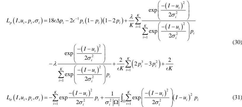
where dt_p and dt_σ are the step sizes for Equations (27) and (28), respectively, and Lu, Lp and Lσ are given by:

(

)

(

)

(

)

(

)

2 2 2 2 2 1 exp 2 , , , 2 exp 2 i i i

u i i i i i

K i _i i i i I u p

L I u p u I u

(7)

(

)

(

)(

)

(

)

(

)

(

)

(

)

(

)

2 2 1 2 1 2 1 2 2 3 2 2 1 2 1 exp 2

, , , 18 2 1 1 2

exp 2

exp

2 ₂ ₂

2 3

exp 2

i

K _i

p i i i i i i i

K i i i i i i K i i i K i i i i i I u

L I u p p p p p

K _I _u

p I u p p K K I u p σ λ σ σ σ λ σ − = = = = _{− −}        = ∆ − − − + _{− −}        _{− −}        − + − + _{− −}       

∑

    (30)

(

)

(

)

2

(

) ( )

2 2

2 2 2

1 1

1

, , , exp exp

2 2

K K

i i

i i i i i i

i i i i i

I u I u

L_σ I u p σ p I u p

σ σ Ω σ

= =   − − − −   = − + −  

Ω _ _

∑

∫

∑

(31)

To start the iteration process, we need to choose the initial values for the ownership functions pi, the

patterns ui and the standard deviations σi. We also need to choose suitable parameters α and λ. The

adopted procedures is: given p xi

( )

, i=1, 2,,K, we take

( ) ( )

0

, ,

i

u x y =I x y if p x y_i

(

,

)

=1 and

( )

0

, 0

i

u x y = if p x y_i

( )

, =0, 0

i

σ =σ.

In Figure 1, a comparison was made between Shen’s model and the proposed model using synthetic images.

Figure 1(a) is the original image, which is a piecewise constant image added with constant Gaussian noise.

Figure 1(b) and Figure 1(c) are the reconstructed images using the proposed model after 10 iterations and 50 iterations resp., while Figure 1(d) to Figure 1(f) are the images reconstructed using Shen’s model after 50 iterations, 100 iterations and 500 iterations, respectively. We see that the result was improved using the proposed model with few iterations. However, when Shen’s model is used very little differences is perceived even when the number of iterations are increased.

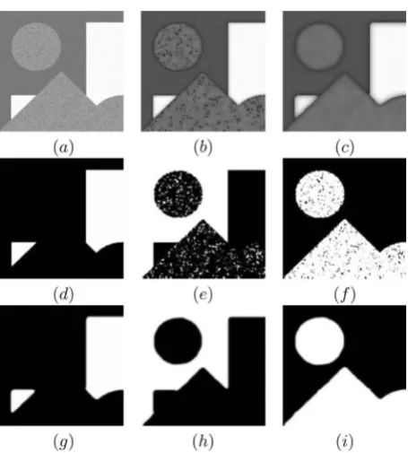
In Figure 2, we present a comparison between variances updated and not updated. The original image Figure 2(a) is a piecewise constant image added with different Gaussian noise for different phases. Figure 2(b) is the reconstructed image when variances are not updated, and Figure 2(c)is the reconstructed image when variances are updated. Figure 2(d), Figure 2(f) are three membership functions obtained with variances not updated, while Figures 2(g)-(i) are three membership functions obtained with variances updated.

Figure 3 shows the bias correction in the proposed model when bias is evident prior to correction in an image. Figure 3(a) is the original image. This image was firstly used by X. Bresson and T.F. Chan in their non-local Chan-Vese model [6]. It is clear that the object (disk) in Figure 3(a) is biased. Figure 3(b) and Figure 3(c) are the membership functions obtained using Shen’s model, while Figure 3(d) and Figure 3(e) are the corre- sponding membership functions obtained using the proposed model by setting different variances in the implementation.

In the following experiments, we tested our model on real images. In Figure 4, we carried out the experiment on the MRI brain image. Figure 4(a) presents the original brain image; Figures 4(b)-(d) are ownerships of white matter, gray matter and CSF, respectively.Figure 4(e) is the reconstructed image; Figures 4(f)-(h) are patterns of the three matters. Figure 5 shows a similar result but with natural scene image.

Finally, we take the experiment on a color image, as shown in Figure 6, whereFigure 6(a) is the original image; Figures 6(b)-(d)are three phases.

[image:7.595.129.538.86.267.2]

(a) (b) (c) (d) (e) (f)

[image:7.595.89.541.631.706.2]

(8)

Figure 2. Comparison between variances updated and not updated.

[image:8.595.200.428.79.332.2]

Figure 3. Comparison between Shen’s model and proposed model using biased image.

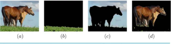
[image:8.595.199.426.357.522.2]

(9)

[image:9.595.172.455.79.213.2]

Figure 5. (a) Original natural image; (b)-(d) Ownerships of different phases; (e) Recon-structed image; (f)-(h) Patterns of different phases.

Figure 6. Experimental result on color image after 300 iterations.

4. Conclusion

In this paper, we extended the idea in paper [35] and developed a soft multiphase segmentation model. The model is a pure Gaussian mixture model. It allows for the choosing of different means and different variances, which leads to a more flexible model. The experiments show that the model is more robust to noise compared with the previous model. Moreover, with the experiment on MRI brain image, we see the advantage of soft segmentation where we can find and calculate partial volume which is very important for brain image segmentation.

Acknowledgements

C.A.Z. Barcelos is partially supported by CNPq-Conselho Nacional de Desenvolvimento Científico e Tec- nológico; Y. Chen is partially supported by NSF grants IIP-1237814 and DMS-1319050.

References

[1] Mumford, D. and Shah, J. (1989) Optimal Approximations by Piecewise Smooth Functions and Associated Variational Problems. Communications on Pure and Applied Mathematics, 42, 577-685. http://dx.doi.org/10.1002/cpa.3160420503

[2] Caselles, V., Kimmel, R. and Sapiro, G. (1997) Geodesic Active Contours. International Journal of Computer Vision,

1, 61-79. http://dx.doi.org/10.1023/A:1007979827043

[3] Paragios, N. and Deriche, R. (2002) Geodesic Active Regions and Level Set Methods for Supervised Texture Segmen-tation. International Journal of Computer Vision, 46, 223-247. http://dx.doi.org/10.1023/A:1014080923068

[4] Zhu, S.C. and Yuille, A. (1996) Region Competition: Unifying Snakes, Region Growing, and Bayes/mdl for Multiband Image Segmentation. IEEE Transaction on Pattern Analysis and Machine Intelligence, 18, 884-900.

http://dx.doi.org/10.1109/34.537343

[5] Osher, S. and Sethian, J.A. (1988) Fronts Propagation with Curvature Dependent Speed: Algorithms Based on Hamil-ton Jacobi Formulations. Journal of Computational Physics, 79, 12-49.

http://dx.doi.org/10.1016/0021-9991(88)90002-2

[6] Vese, L. and Chan. T. (2002) A Multiphase Level Set Framework for Image Segmentation Using the Mumford and Shah Model. International Journal of Computer Vision, 50, 271-293. http://dx.doi.org/10.1023/A:1020874308076

[7] Zhao, B.M.H.-K., Chan, T. and Osher, S. (1996) A Variational Level Set Approach to Multiphase Motion. Journal of Computational Physics, 127, 179-195. http://dx.doi.org/10.1006/jcph.1996.0167

[image:9.595.172.457.249.322.2]

(10)

Approach. Energy Minimization Methods in Computer Vision and Pattern Recognition, 3757, 439-455.

http://dx.doi.org/10.1007/11585978_29

[9] Lie, M.L.J. and Tai, X.C. (2006) A Variant of the Level Set Method and Applications to Image Segmentation. AMS Mathematics of Computations, 75, 1155-1174. http://dx.doi.org/10.1090/S0025-5718-06-01835-7

[10] Chan, T.F., Esedoglu, S. and Nikolova, M. (2006) Algorithms for Finding Global Minimizers of Image Segmentation and Denoising Models. SIAM Journal on Applied Mathematics, 66, 1632-1648. http://dx.doi.org/10.1137/040615286

[11] Bresson, X., Esedoglu, S., Vandergheynst, P., Thiran, J.P. and Osher, S. (2007) Fast Global Minimization of the Active Contour/Snake Model. Journal of Mathematical Imaging and Vision, 28, 151-167.

http://dx.doi.org/10.1007/s10851-007-0002-0

[12] Aujol, J.F. and Chambolle, A. (2005) Dual Norms and Image Decomposition Models. International Journal of Compu- ter Vision, 63, 85-104. http://dx.doi.org/10.1007/s11263-005-4948-3

[13] Aujol, J.F., Gilboa, G., Chan, T. and Osher, S. (2006) Structure-Texture Image Decomposition Modeling Algorithms and Parameter Selection. International Journal of Computer Vision, 67, 111-136.

http://dx.doi.org/10.1007/s11263-006-4331-z

[14] Carter, J. (2001) Dual Methods for Total Variation-Based Image Restoration. Ph.D. Thesis, University of California, Los Angeles.

[15] Chambolle, A. (2004) An Algorithm for Total Variation Minimization and Applications. Journal of Mathematical Im-aging and Vision, 20, 89-97.

[16] Chan, T., Golub, G. and Mulet, P. (1999) A Nonlinear Primal-Dual Method for Total Variation-Based Image Restora-tion. SIAM Journal on Scientific Computing, 20, 1964-1977. http://dx.doi.org/10.1137/S1064827596299767

[17] Chen, S. and Zhang, D. (2004) Robust Image Segmentation Using FCM with Spatial Constraints Based on New Ker-nel-Induced Distance Measure. IEEE Transactions on Systems Man and Cybernetics, 34, 1907-1916.

http://dx.doi.org/10.1109/TSMCB.2004.831165

[18] Mory, B. and Ardon, R. (2007) Fuzzy Region Competition: A Convex Two-Phase Segmentation Framework. Interna-tional Conference on Scale-Space and VariaInterna-tional Methods in Computer Vision, Ischia, 30 May-2 June 2007, 214- 226.

[19] Mory, B., Ardon, R. and Thiran, J.P. (2007) Variational Segmentation Using Fuzzy Region Competition and Local Non-Parametric Probability Density Functions. ICCV 2007, 1-8.

[20] Li, L., Li, X., Lu, H. and Liang, Z. (2005) Partial Volume Segmentation of Brain Magnetic Resonance Images Based on Maximum a Posteriori Probability. Medical Physics, 32, 2337-2345. http://dx.doi.org/10.1118/1.1944912

[21] Pham, D.L. and Prince, J.L. (1998) An Adaptive Fuzzy C-Means Algorithm for the Image Segmentation in the Pres-ence of Intensity Inhomogeneities. Pattern Recognition Letters, 20, 57-68.

http://dx.doi.org/10.1016/S0167-8655(98)00121-4

[22] Bezdek, J.C. (1980) A Convergence Theorem for the Fuzzy ISODATA Clustering Algorithm. IEEE Transactions on Pattern Analysis and Machine Intelligence, PAMI-2, 1-8. http://dx.doi.org/10.1109/TPAMI.1980.4766964

[23] Dunn, J.C. (1973) A Fuzzy Relative of the ISODATA Process and Its Use in Detecting Compact Well-Separated Clus-ters. Journal of Cybernetics, 3, 32-57. http://dx.doi.org/10.1080/01969727308546046

[24] Dempster, A., Laird, N. and Rubin, D. (1977) Maximum Likelihood from Incomplete Data via the EM Algorithm.

Journal of the Royal Statistical Society, Series B, 39, 1-8.

[25] Wells, W., Grimson, E., Kikinis, R. and Jolesz, F. (1996) Adaptive Segmentation of MRI Data. IEEE Transactions on Medical Imaging, 15, 429-442. http://dx.doi.org/10.1109/42.511747

[26] Cahn, J. and Hilliard, J. (1958) Free Anergy of a Non-Uniform System. I. Interfacial Free Energy. The Journal of Che- mical Physics, 28, 258-267. http://dx.doi.org/10.1063/1.1744102

[27] Modica, L. (1987) The Gradient Theory of Phase Transitions and the Minimal Interface Criterion. Archive for Rational Mechanics and Analysis, 98, 123-142.

[28] Modica, L. and Mortola, S. (1977) Un esempio di Gamma-convergenza. Bollettino della Unione Matematica Italiana B,

14, 285-299.

[29] Bourdin, B. and Chambolle, A. (2003) Design-Dependent Loads in Topology Optimization. ESAIM: Control, Optimi-sation and Calculus of Variations, 9, 19-48. http://dx.doi.org/10.1051/cocv:2002070

[30] Burger, M. and Stainko, R. (2006) Phase-Field Relaxation of Topology Optimization with Local Stress Constraints.

SIAM Journal on Control and Optimization, 45, 1447-1466. http://dx.doi.org/10.1137/05062723X

(11)

2, 800-833. http://dx.doi.org/10.1137/080738337

[33] Jung, Y., Kang, S. and Shen, J. (2007) Multiphase Image Segmentation via Modica-Mortola Phase Transition. SIAM Applied Mathematics, 67, 1213-1232. http://dx.doi.org/10.1137/060662708

[34] Li, Y. and Kim, J. (2011) Multiphase Image Segmentation Using a Phase-Field Model. Computers and Mathematics with Applications, 62, 737-745. http://dx.doi.org/10.1016/j.jmaa.2011.05.043

[35] Shen, J. (2006) A Stochastic Variational Model for Soft Mumford-Shah Segmentation. International Journal of Biome- dical Imaging. Published Online.

[36] Posirca, I., Chen, Y. and Barcelos, C.Z. (2011) A New Stochastic Variational PDE Model for Soft Mumford-Shah Seg- mentation. Journal of Mathematical Analysis and Applications, 384, 104-114.

http://dx.doi.org/10.1016/j.jmaa.2011.05.043

[37] Ambrosio, L. and Tortorelli, V.M. (1990) Approximation of Functional Depending on Jumps by Elliptic Functional via t-Convergence. Communications on Pure and Applied Mathematics, 43, 999-1036.

http://dx.doi.org/10.1002/cpa.3160430805

(12)