Cointegration between Investment and Saving in Selected Asian Countries: ARDL Bounds Testing Procedure

(1)

Munich Personal RePEc Archive

Cointegration between Investment and

Saving in Selected Asian Countries:

ARDL Bounds Testing Procedure

Jiranyakul, Komain and Brahmasrene, Tantatape

Purdue University-North Central

2008

Online at

https://mpra.ub.uni-muenchen.de/45076/

(2)

1 Research Report (2008)

Purdue University North Central, Westville, IN, USA

Cointegration between Investment and Saving in Selected Asian Countries:

ARDL Bounds Testing Procedure

Komain Jiranyakul

National Institute of Development Administration, Thailand

Tantatape Brahmasrene

Purdue University North Central, USA

Abstract:

This paper investigates empirically the relationship between savings and investment in Indonesia, Philippines and Thailand by employing the bounds testing procedure. There are not many studies on the Feldstein-Horioka puzzle for the developing countries. Using bounds testing for cointegration, the results do not support a positive correlation between savings and investment in these three Asian countries.

Introduction

Most researchers investigated savings and investment relationship on advanced economies while only a few authors focus on developing nations. This paper explores the relationship between investment and savings in Indonesia, the Philippines and Thailand by examining the Feldstien-Horioka puzzle. The lower saving-investment correlation may be observed in developing countries with bank-based and/or relatively inefficient financial sectors. During the decade from 1997 to 2006, the average investment as percent of GDP in Indonesia, the Philippines and Thailand are 22.1, 18.2 and 25.2 percent, respectively (Table 1). At time of the Asian financial crisis in 1997, the investment level registered 28.3, 24.6 and 33.5 percent in Indonesia, the Philippines and Thailand, respectively. In 2006, investment rates in these three countries were 24.0, 14.3 and 28.6 percent, respectively. On the brighter side, national savings are in good order. The average annual savings as percent of GDP are 30.1, 35.7 and 41.4 percent in Indonesia, the Philippines and Thailand, respectively. The 2006 figures show 33.0, 38.8 and 41.8 percent, compared with the 1997 figures of 35.5, 31.4, 42.0 percent in Indonesia, the Philippines and Thailand, respectively. Figures 1, 2 and 3 provide a casual observation of savings and investment as percent of the gross domestic product. The annual investment and savings fluctuated erratically during the period under study. The Asian financial crisis had devastating effects on investment especially in the Philippines. Only Indonesia and Thailand were able to recover.

Figure 1

Indonesia Savings and Investment as Percent of GDP 1990-2006

0.0% 10.0% 20.0% 30.0% 40.0% 50.0% 60.0%

1990 1991 1992 1993 1994 1995 1996 1997 1998 1999 2000 2001 2002 2003 2004 2005 2006

P

e

rc

e

n

t

o

f

G

D

P

Investment Savings

Figure 2

The Philipines Savings and Investment as Percent of GDP 1990-2006

0.0% 5.0% 10.0% 15.0% 20.0% 25.0% 30.0% 35.0% 40.0% 45.0%

1990 1991 1992 1993 1994 1995 1996 1997 1998 1999 2000 2001 2002 2003 2004 2005 2006

P

e

rc

e

n

t

o

f

G

D

P

Investment Savings

Figure 3

Thailand Savings and Investment as Percent of GDP 1993-2006

0.0% 5.0% 10.0% 15.0% 20.0% 25.0% 30.0% 35.0% 40.0% 45.0% 50.0%

1990 1991 1992 1993 1994 1995 1996 1997 1998 1999 2000 2001 2002 2003 2004 2005 2006

P

e

rc

e

n

t

o

f

G

D

P

Investment Savings

(3)

2

precise evidence whether cointegration exist between these two series.

In this study, the cointegration of investment and savings are assessed using an autoregressive distributed lag (ARDL) and error correction mechanism (ECM) proposed by Pesaran, Shin and Smith (2001). This ARDL-ECM model, also known as ‘bounds testing procedure,’ is used to analyze the level relationships. The common Engle-Ganger cointegration test proposed by Engle and Ganger (1987) requires that all variables be integrated of order one or I(1) and must be known before performing the cointegration test. However, the ARDL procedure can be used without knowing whether all variables are integrated of order zero or one, or mutually cointegrated.

Literature Review

The general literature on Feldstein and Horioka puzzle is presented in this section. Feldstien and Horioka (1980) analyze a sample of 16 countries in the Organization for Economic Cooperation and Development (OECD) during 1960-1974. It shows that domestic investment and savings

are highly correlated with a positive relationship. A positively correlated domestic investment and savings implies low capital mobility. Following the study of Feldstein and Horioka or FH in 1980, most recent studies of the relationship between saving and investment have studied the relationship in the context of capital mobility in the industrialized countries.

Bayoumi (1990) has argued that the use of total investment may lead to spurious correlations with savings that reflect endogenous behavior by private agents. Therefore, it is better to use total business fixed investment. Sarno and Taylor (1998) reexamine the FH approach to measure the degree of international capital mobility. They focus on the difference between the short-run and the long-run saving-investment correlation coefficient and the

[image:3.595.52.552.294.598.2]

effectiveness of the abolition of exchange control. A long period of restrictions on capital flows between the UK and the international economy ended in October 1979. Their results suggest that the short-run saving-investment correlation is significantly higher than the long-run one. The empirical evidence suggests that the UK is financially highly integrated with the world economy after 1979. Sinha and Sinha (1998) study the relationship in ten Latin Table 1. Annual Investment And Savings As Percent of GDP

Year Indonesia Philippines Thailand

Investment(%) Savings(%) Investment(%) Savings(%) Investment(%) Savings(%) 1990 28.0 41.3 22.7 29.1

1991 28.1 40.9 20.2 27.8 1992 27.2 43.6 21.0 27.0

1993 26.2 37.9 23.8 25.5 39.7 43.7 1994 27.5 37.9 23.7 28.2 40.0 44.4 1995 28.4 35.5 22.2 28.6 41.0 45.1 1996 29.5 34.8 23.4 30.7 41.0 43.3 1997 28.3 35.5 24.6 31.4 33.5 42.0 1998 25.7 30.6 21.2 31.0 22.4 42.3 1999 20.6 16.2 19.2 32.7 20.9 41.3 2000 19.8 31.7 18.7 35.0 22.0 42.3 2001 19.3 34.7 18.4 36.3 23.0 41.0 2002 18.5 31.1 17.9 36.6 22.8 41.1 2003 19.3 28.8 16.9 38.0 24.1 40.9 2004 22.4 28.6 16.2 38.9 25.9 40.8 2005 23.6 31.0 15.0 38.8 29.0 40.4 2006 24.0 33.0 14.3 38.8 28.6 41.8 Average

(4)

3

American countries: Colombia, Dominican Republic, Ecuador, El Salvador, Guatemala, Honduras, Jamaica, Mexico, Panama and Venezuela using the cointegration methodology. Their results show a long-run relationship between saving and investment in four countries, Ecuador, Honduras, Jamaica and Panama. The other six countries may face macroeconomic instability in the long run because of the divergence between saving rate and investment rate.

Sinha (2002) investigates the same issue for Japan and ten other Asian countries. Saving and investment rates are cointegrated for Myanmar and Thailand when structural breaks are taken into account. The causality tests show that the growth of the saving rate causes the growth of the investment rate for Malaysia, Singapore, Sri Lanka and Thailand. The reverse causality holds for Hong Kong, Malaysia, Myanmar and Singapore. De Vita and Abbott (2002) used the newly developed ARDL bounds testing to

reexamine savings and investment correlation in the U.S. They found that both savings and investment rates were cointegrated in all sample periods. However, this correlation was weakened during the more liberalized floating exchange rate period. Schmidt (2003) examines the endogeneity of the Australian saving and investment rates. The close association between domestic saving and investment rates may allow for polices which alter domestic saving levels in order to alter domestic investment levels. This presumes an endogenous investment response and that the close association is maintained by movements in national savings. The results highlight the exogeneity of investment and further suggest an endogenous response on the part of Australia's saving rate.

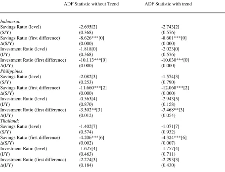
[image:4.595.52.507.135.483.2]

Using UK quarterly data, Abbott and De Vita (2003) examine the nature and degree of the relationship between savings and investment. They find cointegration in all Table 2. ADF Tests For Unit Root

ADF Statistic without Trend ADF Statistic with trend

Indonesia:

Savings Ratio (level) (S/Y)

Savings Ratio (first difference)

∆(S/Y)

Investment Ratio (level) (I/Y)

Investment Ratio (first difference)

∆(I/Y)

-2.695[2] (0.368) -8.626***[0] (0.000) -1.818[0] (0.368) -10.113***[0] (0.000)

-2.743[2] (0.576) -8.601***[0] (0.000) -2.023[0] (0.576) -10.030***[0] (0.000)

Philippines:

∆(S/Y)

∆(I/Y)

-2.082[3] (0.253) -11.660***[2] (0.000) -0.563[4] (0.870) -3.502**[3] (0.012)

-1.574[3] (0.790) -12.060***[2] (0.000) -2.943[5] (0.158) -3.468**[3] (0.054)

Thailand:

∆(S/Y)

∆(I/Y)

-1.402[7] (0.574) -4.206***[6] (0.002) -1.625[4] (0.463) -2.274[3] (0.184)

-1.071[7] (0.932) -4.324***[6] (0.007) -1.757[4] (0.711) -2.293[3] (0.430)

Note: a. The number in brackets is the optimal lag length determined by Schwartz information criterion (SIC). b. The number in parentheses is the p-value provided by MacKinnon (1996).

(5)

4

samples is consistent with the view that the long run relationship between savings and investment is not exclusively dependent upon the level of financial integration. The relationship weakens after the abolition

of UK controls on capital flows in 1979. This suggests the FH framework provides at least a partial measure of the degree of capital mobility. Ho (2003) augments the empirical literature by examining the threshold effect of country size, measured by relative GNP share on the magnitude of saving-retention coefficient. Evidence from a panel of 23 OECD countries indicates that the saving-retention coefficient increases as the relative GNP share becomes larger, which substantially supports the country size argument. Kasuga (2004) employs cross section analysis. The finding suggests that countries which develop primary equity markets have larger savings and investment correlations. The impact of domestic savings on investment depends on financial systems and their development.

Narayan (2005a) tests FH puzzle by applying the bounds testing procedure for China. The saving-investment correlation for China is estimated over the periods 1952-1998 and 1952-1994 (fixed exchange rate regime). Saving

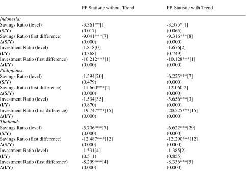
[image:5.595.53.537.175.518.2]

and investment are correlated in China for both the entire sample period and the period of the fixed exchange rate. With high saving-investment correlation, the results conform with the FH hypothesis. In China capital mobility was fairly restricted over the 1952-1994 periods as indicated by the relatively low foreign direct investment. Narayan (2005b) also tests for Japan over the period 1960– 1999. This finding indicates saving and investment are cointegrated for Japan; investment causes saving and saving causes investment; and the long-run coefficient on saving is a moderate correlation rate of 0.68. There is no puzzle Table 3. PP Tests For Unit Root

PP Statistic without Trend PP Statistic with Trend

Indonesia:

∆(S/Y)

∆(I/Y)

-3.361**[1] (0.017) -9.041***[7] (0.000) -1.818[0] (0.368) -10.212***[1] (0.000)

-3.375*[1] (0.065) -9.316***[8] (0.000) -1.676[2] (0.749) -10.128***[1] (0.000)

Philippines:

∆(S/Y)

∆(I/Y)

-1.594[20] (0.479) -11.660***[2] (0.000) -1.534[35] (0.870) -19.747***[15] (0.000)

-6.225***[7] (0.000) -12.060[2] (0.000) -5.656***[3] (0.000) -20.525***[15] (0.000)

Thailand:

∆(S/Y)

∆(I/Y)

-5.706***[7] (0.000) -12.487***[12] (0.000) -1.531[4] (0.511) -8.299***[4] (0.000)

-6.622***[29] (0.000) -12.290***[12] (0.000) -1.385[2] (0.855) -8.336***[5] (0.000) Note: a. The number in brackets is the optimal Newey-West bandwidth.

(6)

5

between saving and investment in the case of Japan, a result contrary to FH (1980). Overall, the empirical results are mixed due in part to the difference in the samples of countries and techniques used in each paper.

Data And Methodology

In order to test the cointegration of investment and savings, the quarterly data of the ratios of savings to GDP and investment to GDP during 1993 to 2006 are retrieved from the International Monetary Fund’s International Financial Statistics. The sample size is 56 quarters in each country from 1993(1) to 2006(4). Recall that in economics, savings equal disposable income minus consumption. Gross national income (GNI) is used as a proxy for disposable income because disposable income data are not available. GNI is the total value of all income generated by a nation's residents from both domestic and international activities. Gross fixed capital formation was a proxy for investment. The bivariate cointegration test is employed to determine the short-run and long-run relationships between savings and investment.

Engle and Granger (EG, 1987) discuss the two-step EG cointegration test in details. In brief, the series are cointegrated or have a long-run relationship if a linear combination of these series exists. According to the two-step EG cointegration test, the unit root test for stationarity property of time series data is determined prior to conintegration test. Dickey and Fuller (1981) propose a unit root test for stationarity of time series called Augmented Dickey-Fuller test or ADF test. This test determines the existence of a unit root of each series. The series are examined whether they are stationary or

integrated of the same order. If the two variables are non-stationary in level but non-stationary in first differences i.e. I(1), cointegration test can be performed. Phillips and Perron (1988) propose another widely used test for unit root, so called the Phillips-Perron Test or PP test. Both ADF and PP tests may yield different results. For example, a mixture of I(0) and I(1) appears in several empirical works. Davidson and MacKinnon (1993) provide the critical values for unit root and cointegration tests.

A common hypothesis is constructed that domestic private investment (I) depends on national saving (S). If savings and investment are integrated of the same order or I(1), there may be a long-run relationship between these two variables. The ordinary least square (OLS) can be performed using the following equation where Y is real GDP.

Table 4. Results Of ARDL-ECM Test For Cointegatrion

Indonesia:

∆It = 0.008 – 0.136It-1 + 0.077St-1 – 0.276∆It-1 + 0.031∆St- 0.051∆St-1

(0.425) (-1.789)* (1.328) (-1.985)** (0.445) (-0.849) Computed F = 1.706, χ2(2) = 1.371 (p=0.504)

Philippines:

∆It = 0.107 – 0.256It-1 – 0.256St-1 – 0.251∆It-1 – 0.180∆It-2 + 0.096∆St + 0.259∆St-1 + 0.501∆St-2

(1.499) (-1.664) (-1.464)* (-1.587) (-1.265) (0.599) (2.132)** (4.004)*** Computed F = 1.407, χ2(2) = 4.650 (p=0.098)

Thailand:

∆It = – 0.154 – 0.130It-1 + 0.450St-1 – 0.189∆It-1 – 0.058∆St – 0.612∆St-1

(-1.283) (-2.064)** (0.427) (-0.650) (-0.319) (-3.781)*** Computed F = 2.136, χ2(2) = 0.630 (p=0.730)

Note: a. The number in parenthesis is t-statistics.

b. *, **, and *** denotes 10, 5, and 1 percent significance level, respectively.

Table 5. The Bounds Critical Value

F-statistics Critical Bounds

4.94 to 5.73 4.04 to 4.78

5 percent 10 percent

Criteria: Conclusion:

Above the upper bound

Between the lower and upper bound Below the lower bound

Cointegrated Inconclusive No cointegration Note: Adapted from Table CI (iii) Case III in

(7)

[image:7.595.62.269.132.235.2]

6

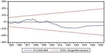
Figure 4. Stability Test for Indonesia

-30 -20 -10 0 10 20 30

95 96 97 98 99 00 01 02 03 04 05 06

[image:7.595.63.267.276.387.2]

CUSUM 5% Significance

Figure 5. Stability Test for the Philippines

-20 -10 0 10 20

96 97 98 99 00 01 02 03 04 05 06

[image:7.595.54.271.423.615.2]

CUSUM 5% Significance

Figure 6. Stability Test for Thailand

-30 -20 -10 0 10 20 30

95 96 97 98 99 00 01 02 03 04 05 06 CUSUM 5% Significance

(1)

t t t

e

Y

S

a

Y

I

+













+

=













1

0

Pesaran, Shin and Smith (2001) proposed a new method for testing cointegration called a conditional autoregressive distributed lag (ARDL) and error correction mechanism (ECM), also known as “ARDL bounds testing procedure.” The ARDL model is specified as

-0.4 0.0 0.4 0.8 1.2 1.6

95 96 97 98 99 00 01 02 03 04 05 06

CUSUM of Squares 5% Significance

-0.4 0.0 0.4 0.8 1.2 1.6

96 97 98 99 00 01 02 03 04 05 06

CUSUM of Squares 5% Significance

-0.4 0.0 0.4 0.8 1.2 1.6

95 96 97 98 99 00 01 02 03 04 05 06 CUSUM of Squares

5% Significance

(2)

t t q

j t j

j p

i t i

i

t Y

S Y

I Y

I _α _β _γ _ϕ _ε

+       ∆ +       ∆ +       ∆ + =      

∆

∑

= −

=1 − 1

0

(8)

7

(3)

t

t q

j t j

j p

i ti

i t t t Y S Y S Y I Y S Y I Y I ε ϕ γ β α α

α +

     ∆ +       ∆ +       ∆ +       +       + =       ∆

∑

= − = − −

− 1 1 1

2 1 1 0

If cointegration exists, replacing the lagged level variables in equation (3) with the one-period lagged residuals from the estimate of equation (1) will yield the error correction term (ECT). The hypotheses are formulated below:

• The null hypothesis of no cointegration among variables:

H

₀

:

α

₀

=

α

₁

=

0 .

• The alternative hypothesis of cointegration:

.

0 :

α

₀

≠

α

₁

≠

a

H

If the F-statistic from Equation (2) is above the critical bound, the null hypothesis of no cointegration is rejected. When the calculated F-statistic is below the lower bound critical value, the null hypothesis is accepted. The F-statistic between the upper and lower bound critical values indicates an inconclusive result.

Empirical Results

The ADF statistics from Table 2 show that savings as a fraction of GDP are nonstationary in level in all cases but their first differences are stationary or I(1) series. On the other hand, investment as a fraction of GDP are I(1) for Indonesia and the Phillipines but not for Thailand.

Thailand’s investment/GDP series contains more than one unit root. For Thailand, the ADF test in Table 2 results differ from the PP test in Table 3. The PP statistics for Thailand show that savings/GDP series is I(0) while investment/GDP series is I(1). This evidence indicates the complex nature of the property of the two variables in the case of Thailand.

The bounds testing procedure consists of the following steps: estimating OLS regression with the first differences of the variables in equation (2), adding lagged level variables and conducting the variable addition test, comparing the F-statistics with the critical values. The bound critical values have two asymptotic critical values. The lower critical value assumes that the regressors are I(0) while the upper critical value assumes that they are I(1).

The criterion for choosing lag length here concludes when the appropriate model ARDL(1,1) shows no further serial correlation at the 5 percent level using Lagrangian Multiplier serial correlation test. The number of lagged differences will increase if the serial correlation is present. The search continues for all combinations of p and q until a model is free from serial correlation. As a result, the lag length of one for Indonesia and Thailand, and two for the Philippines is adopted for the ARDL model in equation (2). Table 4 reports results form bounds testing for cointegration expressed in equation (2). Table 5 summarizes the bounds

critical value for unrestricted intercept with no trend on one regressor and the criteria.

From Table 4, no cointegration exists for all three countries because the computed F-statistics are below the lower bound critical value at 5 and 10 percent significance level (Table 5). Therefore, cointegration does not exist. In Narayan (2005), critical values for the bounds F-test for small sizes are computed ranging from 30-80 observations. Applying the bounds F-test in Narayan (2005) yields similar conclusion when the lag length is 2 and the number of observations is 50. In general, interpret the coefficient of ECM on feedback mechanism is effective in stabilizing external imbalances. However, there is no cointegration in these three cases.

The final models are parsimonious. They pass all the standard diagnostic tests. Serial correlation test shows accepting the null hypothesis of no serial correlation in all ARDL(p,q) models. In addition, there appears to be no structural breaks in all countries (Figures 4-6). The stability test such as the cumulative sum (CUSUM) and cumulative sum square (CUSUMSQ) tests are used to investigate the stability of the equation (2).

Conclusions

By employing the recent time series analysis techniques, the bounds testing shows that investment and savings are not cointegrated only in all cases under study. There is no relationship at level between savings and investment (Table 4). All of these new findings provide further insight into the FH puzzle. This new empirical evidence leads to some implications such as:

• The positive correlation might have been weakened during the more liberalized floating exchange rate period after the financial crisis in the second half of 1997.

• The country size argument (Ho, 2003) may lead to no or negative correlations between savings and investment because these economies are relatively small in terms of real GDP.

• The primary equity markets in these economies are not well developed compared to those of developed countries.

On that last note, while savings to GDP far exceed the investment to GDP ratios (Table 1 and Figures 1-3), the development strategies in these three economies may offer further insight into the degree of capital mobility.

In Indonesia, foreign source of funds have been

(9)

8

overcoming the problem of access to capital and financial need for working capital and growth. To alleviate this problem, the government, in collaboration with the central bank, has been working to pave the way for a further decline in interest rates. Competition among commercial banks with lower rates can encourage firms to rely on domestic savings which in turn provide stimulus growth.

The Philippines government has attempted to attract

and promote local and foreign investments by undertaking reforms aimed at investment liberalization, deregulation and privatization. New policies were implemented during 1999-2004 due to a weakening banking sector and an inability to gain access to domestic credit. The success of these policies might not be materialized in a short period of time even in the presence of an upward trend in domestic savings rates.

With respect to Thailand, improving the overall investment environment is one of the government’s major goals. There has been an implementation of new plans for sustainable growth and stability by strengthening domestic activities and promoting linkages between the domestic and global economies. An improvement in private level investment has occurred in recent years.

Using bounds testing for cointegration, the results do not support a positive correlation between savings and investment in Indonesia, the Philippines and Thailand. In essence, there is no relationship at level between savings and investment. There is relatively high capital mobility in Indonesia, the Philippines and Thailand that may be close to perfect as policy makers attempt to lessen international capital mobility barriers.

References

Abbott, A. and De Vita, G. (2003). Another

piece in the Feldstein–Horioka puzzle. Scottish Journal of

Political Economy, 25, 69-89.

Bayoumi, T. (1990). Saving-investment

correlations: immobile capital, government policy or endogenous behaviour. IMF Staff Papers, 37, 360-87.

Davidson, R., & MacKinnon, J. G. (1993).

Estimation and Inference in Econometrics. Oxford: Oxford

University Press.

De Vita, G., & Abbott, A. (2002). Are saving and investment cointegrated? An ARDL bounds testing approach. Economics Letters, 77(2), 293-299.

Dickey, D. A., & Fuller, W. A. (1981).

Likelihood ratio statistics and autoregressive time series with a unit root. Econometrica, 49, 1057-1072.

Engle, R. E., & Granger, C. W. J. (1987).

Cointegration and error-correction: representation, estmimation, and testing. Econometrica, 55, 251-276.

Feldstein, M. S., & Horioka, C. Y. (1980).

Domestic saving and international capital flows. Economic

Journal, 90(358), 314-329.

Ho, T. W. (2003). The saving-retention

coefficient and country-size: the Feldsteing-Horika puzzle reconsidered. Journal of Macroeconomics, 25(4), 387-396.

Kasuga, H. (2004). Saving-investment

correlations in developing countries. Economics Letters, 83(3), 371-376.

MacKinnon, J. G. (1996). Numerical distribution functions for unit root and cointegration test. Journal of

Applied Econometrics, 11, 601-618.

Narayan, P. K. (2005a). The saving and

investment nexus for China: Evidence from cointegration tests. Applied Economics, 37(17), 1979-1990.

Narayan, P. K. (2005b). The relationship between saving and investment for Japan. Japan and the World

Economy, 17(3),293-309.

Pesaran, M. H., Shin, Y., & Smith, R. J. (2001). Bound testing approaches to the analysis of level relationships. Journal of Applied Econometrics, 16, 289-326.

Phillips, P. C. B., & Perron, P. (1988). Testing for a unit root in time series regression. Biometrika, 75, 335-467.

Sarno, L. and Taylor, M. P. (1998). Exchange

controls, international capital flows and saving-investment correlations in the UK: an empirical investigation.

Weltwirtschaftliches Archiv, 134, 69-97.

Schmidt, M. B. (2003). Savings and investment in Australia. Applied Economics, 35, 99-106.

Sinha, D. (2002). Saving-investment

relationships for Japan and other Asian countries. Japan

and the World Economy, 14, 1–23.