The Thirty-Third AAAI Conference on Artificial Intelligence (AAAI-19)
Online Learning from Data Streams with Varying Feature Spaces
Ege Beyazit
University of Louisiana at Lafayette Lafayette, LA, USA [email protected]
Jeevithan Alagurajah
University of Louisiana at LafayetteLafayette, LA, USA [email protected]
Xindong Wu
University of Louisiana at Lafayette Lafayette, LA, USA
Abstract
We study the problem of online learning with varying fea-ture spaces. The problem is challenging because, unlike tra-ditional online learning problems, varying feature spaces can introduce new features or stop having some features without following a pattern. Other existing methods such as online streaming feature selection (Wu et al. 2013), online learning from trapezoidal data streams (Zhang et al. 2016), and learn-ing with feature evolvable streams (Hou, Zhang, and Zhou 2017) are not capable to learn from arbitrarily varying ture spaces because they make assumptions about the fea-ture space dynamics. In this paper, we propose a novel online learning algorithm OLVF to learn from data with arbitrarily varying feature spaces. The OLVF algorithm learns to clas-sify the feature spaces and the instances from feature spaces simultaneously. To classify an instance, the algorithm dynam-ically projects the instance classifier and the training instance onto their shared feature subspace. The feature space clas-sifier predicts theprojection confidencesfor a given feature space. The instance classifier will be updated by following the empirical risk minimization principle and the strength of the constraints will be scaled by the projection confidences. Afterwards, a feature sparsity method is applied to reduce the model complexity. Experiments on 10 datasets with varying feature spaces have been conducted to demonstrate the per-formance of the proposed OLVF algorithm. Moreover, ex-periments with trapezoidal data streams on the same datasets have been conducted to show that OLVF performs better than the state-of-the-art learning algorithm (Zhang et al. 2016).
Introduction
The goal of learning a classifier in an online setup, where the training instances arrive one by one, has been studied extensively and a wide variety of algorithms have been de-veloped for online learning (Leite, Costa, and Gomide 2010; Yu, Neely, and Wei 2017; Agarwal, Saradhi, and Karnick 2008). These algorithms have made it possible to learn in applications where it is computationally not feasible to train over the entire dataset. Additionally, online learning algo-rithms have been used in applications where the data contin-uously grow over time and new patterns need to be extracted (Shalev-Shwartz and others 2012). However, online learn-ing algorithms assume that the feature space they learn from
Copyright c2019, Association for the Advancement of Artificial Intelligence (www.aaai.org). All rights reserved.
remains constant. On the other hand, in a wide range of ap-plications, feature spaces dynamically change over time. For example in a spam e-mail classification task, each e-mail can have a different set of words and words that are being used in spam e-mails can change over time. In social networks, the features provided by each user can be different than each other. In these scenarios, absence of a feature can also con-vey information and should not be treated as missing data. When the feature space in a data stream keeps changing, we refer the feature space as avarying feature space.
To enable learning from data with varying feature spaces, we propose the Online Learning from Varying Features (OLVF) algorithm, which will also be referred to as ‘the al-gorithm’ in this paper. To learn an instance classifier, the OLVF algorithm projects the existing classifier and the cur-rent instance onto their shared feature subspace, and makes a prediction. Based on the prediction, a loss will be suffered and the classifier will be updated according to an empirical risk minimization principle with adaptive constraints. The algorithm re-weights the constraints based on the confidence of the classifier and the training instance’s projection given the feature space. To learn a feature space classifier, the al-gorithm follows a maximum likelihood principle, using the current feature space information and the output of the in-stance classifier. After each update, a sparsity step is applied to decrease the classifier size. The contributions of this paper can be listed as follows:
• The problem of real-time learning from data where the feature space arbitrarily changes has been studied.
• A new learning algorithm, Online Learning from Varying Features (OLVF), that is capable of learning from varying feature spaces on a single pass is proposed.
• Performance of the OLVF algorithm is empirically vali-dated on 10 datasets in two different scenarios: data with varying feature spaces and trapezoidal data streams.
Related Work
Online Learning
The online learning is performed in consecutive rounds and at each round, the learner is given a training example which can be seen as a question with its answer hidden. The learner makes a prediction on this question and the answer is revealed. Based on the difference between the learner’s prediction and the actual answer, a loss is suffered. The aim of the learner is to minimize the total loss through all rounds. Many different algorithms have been developed for learning in online setting (Tsang, Kocsor, and Kwok 2007; Roughgarden and Schrijvers 2017; Domingos and Hulten 2000; Kuzborskij and Cesa-Bianchi 2017). These algorithms can be broadly grouped into two categories: first-order and second-order methods. First-order algorithms use first-order derivative information for updates (Rosenblatt 1958; Ying and Pontil 2008). Many first order algorithms (Crammer et al. 2006; Gentile 2001; Kivinen, Smola, and Williamson 2004) use the maximum margin principle to find a discrim-inant function that maximizes the separation between dif-ferent classes. By taking the curvature of the space into ac-count, second-order methods improve the convergence and are able to minimize a quadratic function in a finite num-ber of steps (Cesa-Bianchi, Conconi, and Gentile 2005; Crammer, Dredze, and Pereira 2009; Crammer, Kulesza, and Dredze 2009; Wang, Zhao, and Hoi 2016; Orabona and Crammer 2010). Second-order methods are more noise sen-sitive and more expensive than first-order methods, because they require the calculation of the second derivatives. Tra-ditional online learning methods can not learn from varying feature spaces since they assume the feature space they learn from remains the same.
Online Learning from Trapezoidal Data Streams
Online learning from trapezoidal data streams (Zhang et al. 2015; 2016) is closely related to data streams with varying feature spaces. Trapezoidal data streams are streams with a doubly growing nature: the number of instances and the number of features provided by instances can grow simulta-neously. In trapezoidal streams, the current training instance either has the same features as previous instances or ad-ditional new features. In other words the feature space at each iteration contains the feature spaces from previous iter-ations. The proposed algorithmsOLSF−IandOLSF−II learn a linear classifier from trapezoidal data streams by fol-lowing the passive-aggressive update rule. At each iteration, they receive a training instance and try to make a predic-tion. If the prediction is correct, they do not do any classi-fier update, else they update their classiclassi-fier with the weights that minimize the error and are close to the previous clas-sifier weights. While doing this, they also learn additional weights for the new features, if any introduced by the cur-rent training instance. Moreover, sparsity is introduced by applying projection and truncation to the classifier at each round, to decrease the model complexity and improve gen-eralization. HoweverOLSF and its variants can not handle data with varying feature spaces, where the feature space can also shrink and the instances can have completely different sets of features from each other.
Learning with Feature Evolvable Streams
Learning with feature evolvable streams (Hou, Zhang, and Zhou 2017) tackle the problems of classification and regres-sion for data streams where features vanish and new features occur. However, they assume that the feature space evolves in a strictly sequential manner: after the new features arrive, there exists a time period that both the new and old features are available, before some of the old features vanish. Based on this assumption, they use the overlapping time period to learn a projection matrix from old features to the new ones by minimizing a least squares loss. Then to learn a predictor, they propose two methods: weighted combination and dy-namic selection. Weighted combination follows an ensemble strategy by combining the outputs of a set of predictors with weights based on exponential of the cumulative loss. On the other hand, dynamic selection selects the output of the pre-dictor of larger weight with higher probability. Even though learning with feature evolvable streams focuses on feature spaces that can dynamically grow and shrink, the assump-tion of sequential evoluassump-tion is too strong and applicaassump-tion specific. If there is no overlap period of or linear relation-ship between the old and new features, the projection does not carry any useful information. Consequently, the algo-rithm reduces to an ensemble based online learning method with a runtime overhead. Moreover, it is not always compu-tationally feasible to learn a projection matrix and multiple predictors if the data stream is high dimensional.
Learning from data with varying feature spaces is more challenging than the problems stated above since the classi-fier needs to adapt itself to a dynamically changing feature space without any assumptions on the dynamics of the fea-ture space or interactions of feafea-tures. The algorithm needs to continuously learn from data while extracting knowledge when arbitrary features stop being generated as well as new features arrive, in one pass. The existing learning methods are not able to solve learning from varying feature spaces since none of them handle such dynamic and unconstrained feature spaces while learning a classifier.
Preliminaries
In this section, we first present two preliminary concepts that we make use of to design our algorithm: online learn-ing of linear classifiers, and soft-margin classification. Then, we discuss the problem setting for learning binary classifiers from varying feature spaces.
Online Learning of Linear Classifiers
We consider binary classification using linear classifiers. At each roundt, the algorithm receives an instance xt ∈ Rd
and tries to predict the true label yt ∈ {−1,+1} of the instance by using its classifier wt ∈ Rd. Prediction is
done by using the functionyˆt = sign(xt·wt). After pre-diction, the true label of the instance is revealed. Based on the difference between predictionyˆt and true label yt, a loss l(yt,yˆt) is suffered. One of the widely used loss functions is the Hinge loss (Gentile and Warmuth 1999; Wu and Liu 2007; Bartlett and Wegkamp 2008) defined as
between the examplext and the classifierwt. The margin is calculated by y(xt·wt). Because online learning is an incremental task, it is important to minimize the loss while keeping the change to the current model minimum, in order to preserve the knowledge from previous instances. More-over when the data is noisy, forcing the classifier to correctly predict for every instance leads to overfitting and poor gen-eralization. Therefore, it is more preferable to learn a clas-sifier which is able to separate the bulk of the data while ignoring the noise. To accomplish this, a soft decision mar-gin (Shawe-Taylor and Cristianini 2002) is used to let the classifier make a few mistakes. Many online learning algo-rithms combine the constraints stated above and formulate the learning of the weights as an optimization problem:
wt+1= argmin
w: l(yt,ytˆ)≤ξ
1
2kw−wtk
2
+Cξ. (1)
By introducing a slack variable, Equation (1) adds nonlin-earity to the discriminator to allow a certain amount of error to be made. This error is bounded byξ. The parameter C
adjusts the slackness of the constraint. Since real life data is noisy, we use the soft-margin approach to model learning from varying feature spaces.
The Problem Setting and Notation
A feature space that keeps changing on different instances in a data stream is referred to as a varying feature space. We consider the problem of learning a classifier from data with varying feature spaces, by doing single pass over each instance. Let input to the learning algorithm consist of a se-quence of examples (xt, yt)wheret = 1, ..., T. Each in-stance xt ∈ Rxt is a vector that contains an arbitrary set
of features and yt ∈ {−1,+1} is a binary class label for all t. Let wt be the weight vector for the instance classi-fier at round t andyˆt = sign(xt·wt) be the prediction of the instance classifier for the instancext. Letw¯tbe the weight vector for the feature space classifier at roundtand
pt=σ(Rxt·w¯t)is the prediction of the feature space
clas-sifier for the feature spaceRxt.
In data with varying feature spaces, the feature space can dynamically change; new features can be introduced or some of the existing features can cease to exist. At each round
t, when an instance arrives, we divide the explored feature space into three groups: existing, shared and new features. The existing features are only contained by the current clas-sifiers, the new features are only contained by the current instance, and the shared features are the intersection of cur-rent classifiers’ and the curcur-rent instance’s feature spaces. To make a prediction, the learning algorithm projects its cur-rent classifiers and the curcur-rent training instance onto their shared feature space. We denote the projection of a classi-fier at roundtonto the existing feature space aswte, shared feature space aswtsand the new feature space aswtn. This notation also applies for the projections of other vectors such as training instances (xte,xts,xtn), and feature space clas-sifiers (w¯te,w¯ts,w¯nt).
We define a feature spaceRas a binarybag of features vector, where each feature in the shared and new feature
spaces is represented by a one and, each feature in the ex-isting feature space represented by a zero.
Online Learning from Varying Feature Spaces
In this section, we explain the building blocks of the OLVF algorithm and discuss the motivation behind their design. Then, we derive the soft-margin classifier update rules for the instance and feature space classifiers in a binary classi-fication setting. Note that the algorithm can easily be gen-eralized to a multiclass setting by converting the problem to multiple binary classification problems (Bolon-Canedo, Sanchez-Marono, and Alonso-Betanzos 2011), using the One vs Rest or One vs One (S´aez et al. 2014; Xu 2011) strategies. Finally, we combine the building blocks to form the main steps and discuss the running time complexity of the OLVF algorithm.Learning to Predict Projection Confidences
In traditional online learning problems the feature space re-mains constant. When a classifier makes a poor prediction, it needs to be updated aggressively. However in data with vary-ing feature spaces, our instance classifier can make poor pre-dictions because of the unfair conditions caused by varying feature spaces: the instance classifier often needs to predict the labels for instances that belong to feature spaces differ-ent than its own. For example, when our learner receives an instance that does not have some of the features included by the current instance classifier, the learner will not able to use its full potential, since the instance classifier will only be using the features in the shared feature space. Similarly, if the learner receives an instance with new features, the in-stance loses the information provided by the new feature space. Hence, if the instance classifier makes a bad predic-tion, the reason can also be the high difference between the feature spaces of itself and the current instance.
We measure the loss of information after projecting a vec-tor onto a feature space withprojection confidence: proba-bility that the instance classifier makes a correct prediction given the vectors projected feature space. We learn to esti-mate projection confidences by training a feature space clas-sifierw¯t. LetI(y,yˆ)be an indicator function defined as:
I(y,yˆ) =
1, ify= ˆy
0, otherwise (2) We model the probability that the instance classifier wt makes a correct prediction,y = ˆy, given the feature space
Rxtparameterized by the feature space classifierw¯
twith the likelihood function
P(I(yt,yˆt)|Rxt; ¯wt) =
σ(Rxet ·w¯e
t+R xs
t ·w¯s
t+R xn
t ·w¯n
t)
I(yt,ˆyt)+
σ(Rx
e t ·w¯e
t+R xs
t ·w¯s
t+R xn
t ·w¯n
t)
1−I(yt,yˆt). (3)
After taking the negative logarithm of the likelihood func-tion above, we rearrange and define our loss funcfunc-tion to train the feature space classifierw¯tas:
¯
lt(Rxt, I(yt,yˆt),w¯t) =
log(1 +e−I(yt,yˆt) ¯wstR xst
e−I(yt,ˆyt) ¯wntR xnt
Since we learn the feature space classifier in an online set-ting, merely minimizing the loss function can lead to a poor performance. As the learner receives new instances and up-dates the feature space classifier, it is important to preserve the knowledge of previously seen feature spaces. Moreover when a set of new features arrive and need to be added to the current feature space classifier, there can be infinitely many solutions because of the lack of information about those new features. To avoid overfitting, we need to learn the smallest weights possible that minimize the loss. Also, because real-life data is noisy, we want our algorithm to follow a soft-margin strategy to avoid poor generalization. As a result, we formulate the problem of learning the feature space classifier as constrained optimization, using the loss function defined in Equation (4):
¯
wt+1= argmin ¯
w=[ ¯we,w¯s,w¯n]: ¯
lt≤ξ,ξ≥0
1 2kw¯
e−w¯e tk
2
+
1 2kw¯
s−w¯s tk
2
+1 2kw¯
nk2
+ ¯Cξ, (5)
Note that we use the slack variableC¯to bound the loss¯lt. We solve the optimization problem with the inequalities¯lt ≤ξ andξ ≥ 0 defined in Equation (5) by using a Lagrangian function with K.K.T. conditions (Luo and Yu 2006):
L( ¯w, τ, α, ξ) = 1 2kw¯
e−w¯e tk
2
+1 2kw¯
s−w¯s tk
2
+
1 2kw¯
nk2
+ ¯Cξ+τ(¯lt−ξ)−αξ, (6)
whereτandαare Lagrange multipliers. Setting the deriva-tives ofL( ¯w, τ, α, ξ)with respect tow¯e,w¯s,w¯n andξ, we obtain the following conditions:
¯
we= ¯wet
¯
ws= ¯wst+τ
∂¯lt(Rxt, I(y
t,yˆt),w¯t)
∂w¯s
wn=−τ∂
¯
lt(Rxt, I(y
t,yˆt),w¯t)
∂w¯n
α=C−τ,
where
∂¯lt(Rxt, I(y
t,yˆt),w¯t)
∂w¯s =
− log(e
−I(yt,yˆt)( ¯wstR xst+ ¯wn
tR xnt)
)
log(1 +e−I(yt,yˆt)( ¯wstR xst+ ¯wn
tR xnt)
)I(yt,yˆt)R xs
t, (7)
and
∂¯lt(Rxt, I(y
t,yˆt),w¯t)
∂w¯n =
− log(e
−I(yt,yˆt)( ¯wstR xst+ ¯wn
tR xnt)
)
log(1 +e−I(yt,ˆyt)( ¯wstRxst+ ¯wtnRxnt))
I(yt,yˆt)Rx
n t (8)
Using the conditions and partial derivatives defined above, we obtain the following representation of our problem and
findτ:
L(τ) = 1 2τ 2
∂¯lt
∂w¯s
2 +1 2τ 2
∂¯lt
∂w¯n
2 +
τ¯lt(Rxt, I(yt,yˆt),w¯t) (9)
τ=min{C,−
¯
lt(Rxt, I(y
t,yˆt),w¯t)
∂¯lt
∂w¯s
2 +
∂¯lt
∂w¯n
2 }. (10)
To make a prediction given an instance xt, the learner makes projections of both the instance classifier and the in-stance onto the current shared feature space. We use the feature space classifier w¯t to estimate the projection con-fidences and adaptively re-weight the different parts of the objective function corresponding to the different pieces of the instance classifier weightswt = [wet, wst, wnt]. This re-weighting strategy helps to adjust the priorities of each con-straint in the objective function, scales the regularization weights for each instancext, and improves the learning con-vergence.
Learning to Classify Instances from Varying
Feature Spaces
In order to adapt the instance classifier to the dynamic na-ture of the varying feana-ture spaces, we modify the Hinge loss by using the projections of the instance classifier and the in-stance:
lt=max{0,1−y(xts·ws)−y(xtn·wn)}. (11) Motivated by the same reasons discussed for the objective function defined in Equation (5), we formulate the problem of learning the instance classifier from varying features as
wt+1= argmin
w=[we,ws,wn]: lt≤ξ,ξ≥0
1 2kw
e
−wtek
2
+
1 2p
w t kw
s
−wtsk
2
+1 2p
x tkw
n
k2+Cξ, (12) wherepw
t =σ(Rwt·w¯t)is the projection confidence of the instance classifierwtandpxt = σ(Rxt ·w¯t)is the projec-tion confidence of the instancext. Note that the objectives for ws and wn are weighted using these projection con-fidences. When the projection confidence of the classifier onto the shared subspacepw
t is close to 1, then the shared feature space is not very different than the feature space of the current classifier. Therefore, the objective of minimizing
kws−w tsk
2
is important in order to remember the informa-tion received from previous instances. Moreover if the pro-jection confidence of the training instance onto the shared subspacepx
tis close to 1, the objective of minimizingkwnk
2
rules:
we=wte
ws=wts+τ pwtytxts
wn =τ pxtytxtn
α=C−τ.
Using these conditions, we obtain the following representa-tion of our problem and findτ:
L(τ) = 1 2τ
2(pw t)
2
kxtsk
2
+1 2τ
2(px t)
2kx
tnk
2
+
τ(1−yt(wts·xts)), (13)
τ =min{C, −lt
kxtk
2}. (14)
After rearranging, we can define the update strategy as:
wt+1= [wet+1, w
s t+1, w
n t+1] =
[we, wts+min{Cpwtytxts,
pw tltytxts
kxtk
2 },
min{Cpxtytxtn,
px tltytxtn
kxtk
2 }]. (15)
Model Sparsity
Because the feature space can dynamically change, the num-ber of features kept in the classifiers are not bounded. In its current design, the learner keeps remembering even if the features stop being generated. This can act as a bias on feature space and instance classifier weights when the fea-tures are reintroduced. Moreover, when vanishing feafea-tures re-emerge, there is a possibility that their meanings are dif-ferent. As a result, this bias can lead to a poor performance. Furthermore, because there is no feature selection mecha-nism in the learner, the learner keeps using even the least important features. Therefore, to improve the memory us-age and running time efficiency, we do not want to keep the classifier weights for every feature received by the learner. Simply truncating the smallest weights from the instance classifier leads to poor performance because it introduces a sudden change to the result of the dot product. On the other hand, the feature space classifier can tolerate this change be-cause of the saturating sigmoid function. Therefore to spar-sify the instance classifier, we introduce the following pro-jection step before truncation:
wt:=min{1,
λ wt·w¯t
}wt, (16)
whereλis a regularization parameter. With a ratio ofB, we truncate the smallest elements from the classifiers. Sincew¯t carries the information of which features contribute to the classification task, we use it to scale the weights of the in-stance classifier. This strategy helps to identify and truncate the features that are either redundant or vanishing.
Algorithm 1:The OLVF Algorithm
Input : C,C >¯ 0: Loss bounding parameters
λ >0: Regularization parameter
B ∈(0,1]: Proportion of selected features Initialize:w1= (0, ...,0)∈Rx1
Initialize:w1¯ = (0, ...,0)∈Rx1
1 fort = 1,2,... Tdo
2 Receive the current instancext∈Rxt
3 Identify the shared feature spaceRs=Rwt∩xt
4 Projectwt, xtontoRs:wts, xts
5 Predict the class label:yˆt=sign(wts·xts) 6 Receive the correct label:yt∈ {+1,−1} 7 Update feature space classifier withyt,yˆt,Rxt;
using Equation (7).
8 Predict the projection confidences: 9 pwt =σ(Rwt·w¯
t) 10 pxt =σ(Rxt·w¯t)
11 Update the instance classifier withxt, yt, pwt, pxt; using Equation (15).
12 Projectwt+1using Equation (16) andλ. 13 Truncatewt+1andw¯t+1usingB.
14 end
Time Complexity of OLVF
The pseudocode of our online learning from varying features (OLVF) algorithm is shown in Algorithm 1. The time com-plexity of the OLVF algorithm is as follows. Assuming at roundt,|wt| = |w¯t|is the number of features in the cur-rent classifiers, |xt|is the number of features arrived with the training instance, and|Rs|is the number of features in
the shared feature space. Since the operations are being done for both the weight vectors and the current training instance, the time complexity for identifying the shared feature space and projecting the weight vectors with the training instance onto their shared feature space is O(|wt|+|xt|). The time complexity for making a prediction, calculating the projec-tion confidences and suffering losses is O(|Rs|), because all
of these steps use the shared feature space. Finally, the time complexity for the sparsity step is O(|wt|), since the size of the instance classifier is always equal to the size of the fea-ture space classifier. For a single round, the worst case time complexity of the OLVF algorithm isO(|wt|+|xt|+|Rs|).
Because|Rs|is always less than|w
t|+|xt|, we can further simplify the complexity asO(|wt|+|xt|). Considering the fact that at any roundtthe feature sets ofwtandxtcan be completely disjoint, we do not apply further simplification for the time complexity. In other words, the running time of the algorithm linearly scales with the number of features that are being used at each roundt.
Experiments
Table 1: Numbers of samples and features of 10 datasets. Dataset # Samples # Features
wpbc 198 34
ionosphere 351 35
wdbc 569 31
wbc 699 10
german 1,000 24
svmguide3 1,234 21
spambase 4,601 57
magic04 19,020 10
imdb 25,000 7500
a8a 32,561 123
classifier incrementally and only a single pass is allowed. Similarly, the classifier does not have any initial knowledge about the full feature space. We use 9 different UCI datasets to simulate these scenarios. Additionally, we demonstrate the effectiveness of the proposed sparse strategy. Finally we evaluate the performance of OLVF using the real-world dataset IMDB movie reviews (Maas et al. 2011). The num-bers of instances and features for each dataset are listed in Table 1. In all experiments, we measure the performance in terms of the average prediction accuracy on 20 random per-mutations of each dataset. The parametersCandC¯are cho-sen using grid search.
Experiments on Varying Feature Spaces
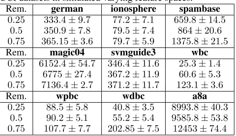
We simulate data with varying feature spaces by randomly removing features from every training instance. We denote the ratio of features removed from each training instance as removing ratio (Rem.). At each round, we apply a ran-dom permutation to the complete dataset and ranran-domly re-move the features. We conduct two different types of ex-periments for varying features. The first set of exex-periments measure the performance of the proposed algorithm in vary-ing feature spaces usvary-ing removvary-ing ratios of 0.25,0.5 and 0.75. The second set of experiments show the trade-off be-tween the accuracy and the sparsity of the classifier, in data with varying feature spaces using0.25as the removing ra-tio.1) Experiments using different removing ratios:We test the performance of the proposed algorithm using 3 differ-ent removing ratios:0.25,0.5and0.75. If the removing ra-tio for a varying feature space is0.25, then1/4 of the fea-tures are randomly removed from each training instance, and so on. Table 2 shows the average number of wrong predic-tions made by OLVF with different removing ratios on 9 UCI datasets. For all datasets, OLVF achieves higher accu-racy on the experiments with smaller removing ratio. This is expected since a small removing ratio means a high number of features sent to the classifier.2) Experiments on sparse and non-sparse OLVF:We observe the trade-off between us-ing sparse classifiers to decrease the time and space usage, and using the full feature space to increase the accuracy. To demonstrate the effect of the sparsity step, we set the remov-ing ratio to0.25while simulating the varying feature spaces. Table 3 shows the average number of errors made by OLVF and sparse OLVF. Table 4 shows the number of features
Table 2: Average number of errors made by OLV F on 9 UCI datasets in simulated varying feature spaces.
Rem. german ionosphere spambase 0.25 333.4±9.7 77.2±7.1 659.8±14.5
0.5 350.9±7.8 79.5±7.4 864±20.6 0.75 365.15±3.6 79.7±5.9 1375.8±21.5
Rem. magic04 svmguide3 wbc
0.25 6152.4±54.7 346.4±11.6 25.3±1.4 0.5 6775±27.4 367.2±11.9 60.6±5.3 0.75 7136.4±2.7 371.2±11.7 123.1±3.6
Rem. wpbc wdbc a8a
0.25 88.5±5.8 40.8±3.5 8993.8±40.3 0.5 90.2±5.1 55.2±5.4 9585.8±53.8 0.75 107.7±7.7 202.85±7.5 12453±74.4
Table 3: Average number of errors made by non-sparse
OLV F and sparseOLV F on 9 UCI datasets in simulated varying feature spaces.
Alg german ionosphere spambase
ns. 333.4±9.7 77.2±7.1 659.8±14.5
s. 358±9.2 79±15.9 825.1±42.7
Alg magic04 svmguide3 wbc
ns. 6154±47.1 367.4±11.6 25±1.4
s. 6621.6±46.6 361.4±20.7 32.3±2.6
Alg wpbc wdbc a8a
ns. 90.2±5.1 39.6±5.2 8933.2±28.5
s. 97.4±4.6 131±7.9 8588.6±575.3
used by the non-sparse and sparse versions of the OLVF algorithm, along with their parameter settings. We can see that with datasets german, ionosphere, spambase, magic04, svmguide3, wbc and a8a sparse and non-sparse versions of the proposed algorithm perform similarly, while the sparse version of the algorithm uses a smaller subset of the pro-vided feature space. With the wpbc dataset, the sparse ver-sion of the algorithm demonstrates a more consistent perfor-mance because the sparse strategy helps to reduce the noise and avoid overfitting. In the wdbc dataset, the sparse version of the proposed algorithm performs similarly to the non-sparse version. However, it follows a lower accuracy trend by∼10%because wdbc has a relatively less number of in-stances and less redundant features after randomly removing 1/4 of the features to simulate varying feature spaces.
Table 4: Parameters used by the sparse OLVF algorithm.
Dataset B C C
wbc 0.6 1 0.01
svmguide3 0.4 0.1 0.001 wpbc 0.7 0.0001 0.01 ionosphere 0.1 0.01 0.1
magic04 0.6 0.1 0.0001 german 0.5 0.01 0.001 spambase 0.3 0.01 0.001
wdbc 0.9 1 0.1
Table 5: Average number of errors made by OLSF and
OLV F on 9 UCI datasets in simulated trapezoidal data streams, and on the IMDB dataset.
Algorithm german ionosphere
OLSF 385.5±10.2 57.9±4.7
OLV F 329.2±9.8 51.8±3.1
Algorithm magic04 svmguide3
OLSF 6147.4±65.3 361.7±29.7
OLV F 5784.0±52.7 351.6±25.9
Algorithm wpbc wdbc
OLSF 87.9±5.6 52.9±4.5
OLV F 78.2±5.5 45.4±2.9
Algorithm spambase wbc
OLSF 993.5±25 48.1±12.6
OLV F 825.8±20.2 31.1±2.8
Algorithm a8a imdb
OLSF 9420.4±549.9 7851.0±51.4
OLV F 8649.8±526.7 4474.2±39.1
Experiments on Trapezoidal Data Streams
We compare the prediction accuracy of OLVF withOLSF algorithms (Zhang et al. 2016) on trapezoidal data streams. For each dataset, we use the version ofOLSF that performs the best to compare with our algorithm. For the sparsity step, we use the same λand B parameters as in (Zhang et al. 2016). We used grid search to find the best C and C¯ for each dataset. To simulate trapezoidal data streams, we split each dataset into 10 chunks where the number of features included by each chunk increases as the data flows in. For example, instances in the first chunk have the first 10 per-cent of features, instances in the second chunk have the first 20 percent of features and so on. Table 5 shows the average numbers of errors with variances of the OLVF and theOLSF algorithms in trapezoidal streams. Note that because the ex-isting and shared feature spaces in trapezoidal data streams never change, the only component that is effective while re-weighting the objective function is the projection confidence of the current training instance. From these experiments, we observe that our OLVF achieves higher prediction accuracy while learning classifiers with the same sparsity as OLSF, because of its feature space adaptive constraint re-weighting strategy. In Table 5 we observe that in addition to lower num-bers of errors in 9 UCI datasets, the standard deviation of the errors made by OLVF in 20 rounds is also lower than the OLSF algorithms. This shows that OLVF has consistently better performance than the OLSF algorithms on the 9 UCI datasets.
Application to Real-World Varying Feature Spaces
In IMDB Movie Reviews dataset, the task is to classify each movie review, provided in raw text, into positive or negative sentiment. Each new movie review can include words that the learner have never seen, or exclude the words exist in the learners feature space. Hence, we can formulate the prob-lem as learning from varying feature spaces and use OLVF. The problem can also be seen as learning from trapezoidal data streams by assuming non-existing features are missing
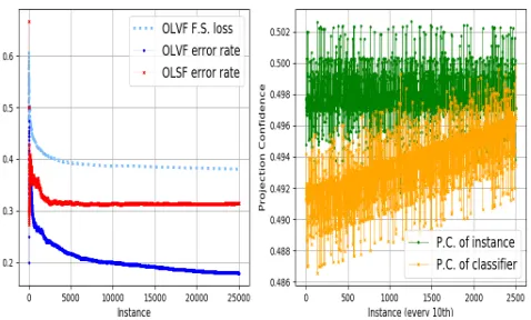
Figure 1: Mean error rates ofOLV FandOLSF algorithms as the data streams in (left), and projection confidences esti-mated by the feature space classifier (right).
data. We evaluate these two approaches by comparing the prediction accuracies of OLVF andOLSF algorithms. For both algorithms, we setB’s to 0.1 and find their best setting for theCandC¯parameters by using grid search. We set the C to 0.1, andC¯to10−5.
Table 5 shows that average number of wrong predictions made by OLVF is lower than OLSF. Moreover, Figure 1 (left) shows that OLVF has a faster learning trend and higher accuracy thanOLSF because of its feature space adaptive constraint weighting strategy. Figure 1 (left) also shows that the loss suffered by the feature space classifier of OLVF de-creases as the data streams in. This indicates that the model learns how to classify feature spaces as it receives more in-stances. Figure 1 (right) shows the change of projection con-fidence predictions made by the feature space classifier. Note that the projection confidences randomly fluctuate because each instance comes from an arbitrary feature space. Addi-tional to the fluctuations, the projection confidence of the instance classifier has an increasing trend. This is because the instance classifier learns new features and new informa-tion relevant to its existing features, therefore becomes more confident against unknown features as the data streams in.
Conclusion
Acknowledgments
This research is supported by the US National Science Foun-dation (NSF) under grants 1652107 and 1763620.
References
Agarwal, S.; Saradhi, V. V.; and Karnick, H. 2008. Kernel-based online machine learning and support vector reduction. Neurocomputing71(7-9):1230–1237.
Bartlett, P. L., and Wegkamp, M. H. 2008. Classification with a reject option using a hinge loss. Journal of Machine Learning Research9(Aug):1823–1840.
Bolon-Canedo, V.; Sanchez-Marono, N.; and Alonso-Betanzos, A. 2011. Feature selection and classification in multiple class datasets: An application to kdd cup 99 dataset. Expert Systems with Applications38(5):5947–5957. Cesa-Bianchi, N.; Conconi, A.; and Gentile, C. 2005. A second-order perceptron algorithm. SIAM Journal on Com-puting34(3):640–668.
Crammer, K.; Dekel, O.; Keshet, J.; Shalev-Shwartz, S.; and Singer, Y. 2006. Online passive-aggressive algorithms. Journal of Machine Learning Research7(Mar):551–585. Crammer, K.; Dredze, M.; and Pereira, F. 2009. Exact con-vex confidence-weighted learning. InAdvances in Neural Information Processing Systems, 345–352.
Crammer, K.; Kulesza, A.; and Dredze, M. 2009. Adap-tive regularization of weight vectors. InAdvances in Neural Information Processing Systems, 414–422.
Domingos, P., and Hulten, G. 2000. Mining high-speed data streams. In Proceedings of the sixth ACM SIGKDD international conference on Knowledge Discovery and Data Mining, 71–80. ACM.
Gentile, C., and Warmuth, M. K. 1999. Linear hinge loss and average margin. InAdvances in Neural Information Pro-cessing Systems, 225–231.
Gentile, C. 2001. A new approximate maximal margin clas-sification algorithm.Journal of Machine Learning Research 2(Dec):213–242.
Hou, B.-J.; Zhang, L.; and Zhou, Z.-H. 2017. Learning with feature evolvable streams. InAdvances in Neural Informa-tion Processing Systems, 1417–1427.
Kivinen, J.; Smola, A. J.; and Williamson, R. C. 2004. On-line learning with kernels.IEEE Transactions on Signal Pro-cessing52(8):2165–2176.
Kuzborskij, I., and Cesa-Bianchi, N. 2017. Nonparametric online regression while learning the metric. InAdvances in Neural Information Processing Systems, 667–676.
Leite, D.; Costa, P.; and Gomide, F. 2010. Evolving granular neural network for semi-supervised data stream classifica-tion. InNeural Networks (IJCNN), The 2010 International Joint Conference on, 1–8. IEEE.
Luo, Z.-Q., and Yu, W. 2006. An introduction to convex op-timization for communications and signal processing.IEEE Journal on Selected Areas in Communications24(8):1426– 1438.
Maas, A. L.; Daly, R. E.; Pham, P. T.; Huang, D.; Ng, A. Y.; and Potts, C. 2011. Learning word vectors for sentiment analysis. In Proceedings of the 49th Annual Meeting of the Association for Computational Linguistics: Human Lan-guage Technologies, 142–150. Portland, Oregon, USA: As-sociation for Computational Linguistics.
Orabona, F., and Crammer, K. 2010. New adaptive algo-rithms for online classification. InAdvances in Neural In-formation Processing Systems, 1840–1848.
Rosenblatt, F. 1958. The perceptron: A probabilistic model for information storage and organization in the brain. Psy-chological Review65(6):386.
Roughgarden, T., and Schrijvers, O. 2017. Online predic-tion with selfish experts. InAdvances in Neural Information Processing Systems, 1300–1310.
S´aez, J. A.; Galar, M.; Luengo, J.; and Herrera, F. 2014. Analyzing the presence of noise in multi-class problems: al-leviating its influence with the one-vs-one decomposition. Knowledge and Information Systems38(1):179–206. Shalev-Shwartz, S., et al. 2012. Online learning and online convex optimization. Foundations and Trends in Machine Learning4(2):107–194.
Shawe-Taylor, J., and Cristianini, N. 2002. On the gener-alization of soft margin algorithms. IEEE Transactions on Information Theory48(10):2721–2735.
Tsang, I. W.; Kocsor, A.; and Kwok, J. T. 2007. Simpler core vector machines with enclosing balls. InProceedings of the 24th International Conference on Machine Learning, 911–918. ACM.
Wang, J.; Zhao, P.; and Hoi, S. C. 2016. Soft confidence-weighted learning.ACM Transactions on Intelligent Systems and Technology (TIST)8(1):15.
Wu, Y., and Liu, Y. 2007. Robust truncated hinge loss sup-port vector machines. Journal of the American Statistical Association102(479):974–983.
Wu, X.; Yu, K.; Ding, W.; Wang, H.; and Zhu, X. 2013. Online feature selection with streaming features. IEEE Transactions on Pattern Analysis and Machine Intelligence 35(5):1178–1192.
Xu, J. 2011. An extended one-versus-rest support vec-tor machine for multi-label classification. Neurocomputing 74(17):3114–3124.
Ying, Y., and Pontil, M. 2008. Online gradient descent learn-ing algorithms.Foundations of Computational Mathematics 8(5):561–596.
Yu, H.; Neely, M.; and Wei, X. 2017. Online convex opti-mization with stochastic constraints. InAdvances in Neural Information Processing Systems, 1428–1438.
Zhang, Q.; Zhang, P.; Long, G.; Ding, W.; Zhang, C.; and Wu, X. 2015. Towards mining trapezoidal data streams. In Data Mining (ICDM), 2015 IEEE International Conference on, 1111–1116. IEEE.