Ordinal data supervised classification with Quantile-based and other classifiers

(1)

Alma Mater Studiorum

Università di Bologna

DOTTORATO DI RICERCA IN SCIENZE STATISTICHE CICLO XXX Settore Concorsuale: 13/D1

Settore Scientico Disciplinare: SECS-S/01

Ordinal data supervised classication

with Quantile-based and other classiers

Presentata da: Lorenzo Mancini

Coordinatore Dottorato:

Prof.ssa Alessandra Luati

Supervisore:

Prof.ssa Cinzia Viroli

Co-Supervisore:

Prof. Christian Hennig

(2)

(3)

Alma Mater Studiorum

University of Bologna

PHD DEGREE IN STATISTICAL SCIENCES CYCLE XXX Competition eld: 13/D1

Academic discipline: SECS-S/01

Ordinal data supervised classication

with Quantile-based and other classiers

Presented by: Lorenzo Mancini

Ph.D. Director:

Prof. Alessandra Luati

Supervisor:

Prof. Cinzia Viroli

Co-Supervisor:

Prof. Christian Hennig

(4)

(5)

Abstract

The aim of this research project is to propose a new method for supervised classication problems where the input features are ordinal. Ordinal data are preponderant in many research elds. They directly arise when the ob-servations fall into separate distinct but ordered categories and they are very common in surveys where answers are listed as Likert scales. Typically, they are coded as equally spaced values and sometimes they are analyzed as nu-merical values. These choices may not necessarily correspond to the real distribution of the data.

The objectives of the study have been accomplished according to several steps. The rst phase consisted of an exhaustive analysis of the state of art of the statistical literature with the aim of identifying the various approaches to ordinal data analysis, the related limitations, and possible advantages. We have then proposed to operate in the framework of Generalized Linear Latent Variable Models (GLLVM), considering the response function approach with a single latent variable Beta distributed. Our scope in using this method is to shift from a set of ordinal features to a single continuous feature, which well adapt the data, in order to directly apply the standard classication methods.

A dedicated EM algorithm has been developed on the basis of this theoretical framework using the statistical software R.

Finally, we have compared our approach with several scoring methods through a wide simulation study. The scoring methods that we have considered in the simulation study are: the raw scores, the ridits, the blom scores, the normal median scores and the conditional mean scores. These methods, although have a long history in literature, have never been used for classication pur-pose.

In addition we present an example of the application of the proposed ap-proach to real world business data problem.

(6)

(7)

Sommario

Il lavoro di ricerca ha l'obiettivo di individuare una metodologia statistica per la classicazione supervisionata di unità statistiche misurate da un insieme di variabili ordinali. In generale, si parla di variabili ordinali ogniqualvolta il carattere assume stati discreti ma ordinabili. Questo tipo di dati è molto dif-fuso in diverse aree di ricerca e, in particolare, è molto comune nei sondaggi, dove le categorie di risposta sono elencate tramite scale Likert. Tipicamente, le categorie associate a queste variabili sono codicate attraverso apposite etichette. Le etichette corrispondono solitamente a valori numerici progres-sivi ed equi-distanziati che riettono l'ordine delle categorie. In fase di anal-isi non è però appropriato trattare questi dati come valori numerici reali, in quanto, così facendo, si andrebbe ad introdurre una distanza tra categorie che potrebbe non corrispondere a quella eettiva.

Il progetto di ricerca si articola in diverse fasi. Inizialmente, viene eettuata un'analisi esaustiva dello stato dell'arte della letteratura, per identicare i vari approcci all'analisi dei dati ordinali, valutandone i limiti e i vantaggi. Successivamente, sulla base dei risultati di questa analisi, viene proposto un metodo basato sull'approccio response function, nel contesto dei modelli gen-eralizzati a variabili latenti. A dierenza del metodo classico, che prevede variabili latenti normalmente distribuite, la nuova metodologia proposta con-sidera una singola variabile latente con distribuzione Beta, poiché fornisce specici vantaggi in termini di ecienza computazionale e di adattamento ai dati. L'obiettivo è, sostanzialmente, di spostare il problema della classi-cazione da un insieme di variabili ordinali ad una singola variabile continua, in modo da applicare i metodi di classicazione standard.

Sulla base di questo quadro teorico di riferimento è stato sviluppato un al-goritmo EM, utilizzando il software statistico R.

Inne, l'approccio proposto è confrontato, attraverso un ampio studio di sim-ulazione, con diversi metodi di scoring, in particolare: raw scores, ridits, blom scores, normal median scores e conditional mean scores. Questi metodi non sono mai stati usati per scopi di classicazione, sebbene abbiano una lunga tradizione nella letteratura.

Si presenta, in aggiunta, un'applicazione del metodo discusso ad un problema di classicazione su dati reali.

(8)

(9)

Acknowledgements

First and foremost I would like to thank my advisor Prof. Cinzia Viroli for her constant support of my Ph.D study and research, for her contributions of time, motivation, enthusiasm, gentle encouragement and faith in me during the dissertation process.

Her guidance was invaluable and helped me in all the time of research and writing of this thesis.

Besides my advisor, I would like to thank my co-supervisors Prof. Christian Hennig for inviting me at the University College of London. This has been a great opportunity and helped me to grown as researcher. I thank him for the academic support, for his insightful comments and for all the illuminating discussions we had.

Lastly, I would like to thank my family for all their love and encouragement. For my parents who raised me with a love of science and supported me in all my pursuits.

(10)

(11)

List of Figures

1.1 Floor eect . . . 7

2.1 Comparison of scoring methods with raw scores . . . 28

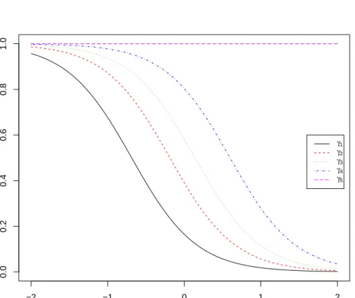
3.1 Cumulative Probabilities . . . 40

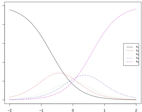
3.2 Response Probabilities . . . 41

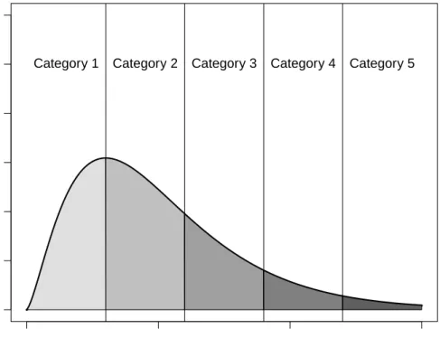
3.3 Ordinal categories from a χ2 underlying distribution . . . 43

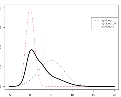
3.4 Underlying mixture distribution . . . 44

4.1 LDA decision boundaries . . . 61

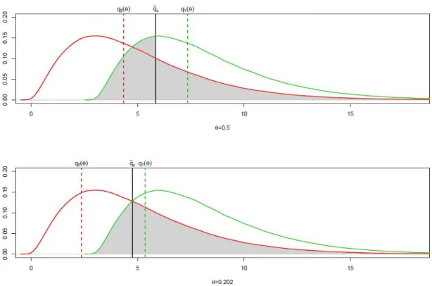
4.2 Location shifted χ2 distributions with total misclassication probability . . . 67

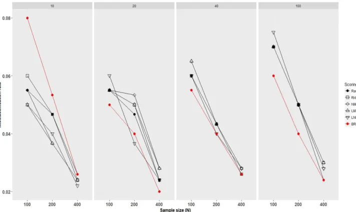
5.1 Quantile-based results for scenario 1 (C= 5 categories) . . . . 75

5.4 Quantile-based results for mixture scenario (C = 5 categories) 78 5.5 LDA results for scenario 1 (C = 5 categories) . . . 82

5.6 QDA results for scenario 1 (C = 5 categories) . . . 83

5.7 SVM results for scenario 1 (C = 5 categories) . . . 84

5.8 Naive Bayes classier results for scenario 1 (C = 5 categories) 85 5.9 Comparison of classiers on the scoring methods for scenario 1 (C = 5 categories) . . . 89

5.10 Comparison of classiers on the scoring methods for scenario 2 (C = 5 categories) . . . 90

5.11 Comparison of classiers on the scoring methods for scenario 3 (C = 5 categories) . . . 91

5.12 Comparison of classiers on the scoring methods for mixture scenario (C = 5 categories) . . . 92

(16)

xii LIST OF FIGURES

A.1 Quantile-based results for scenario 1 (C = 3 categories) . . . . 109

A.4 Quantile-based results for mixture scenario (C = 3 categories)112 A.5 Quantile-based results for scenario 1 (C = 357 categories) . . . 114

A.6 Quantile-based results for scenario 2 (C = 357 categories) . . . 115

A.7 Quantile-based results for scenario 3 (C = 357 categories) . . . 116

A.8 Quantile-based results for mixture scenario (C = 357 cate-gories) . . . 117

A.9 LDA results for scenario 2 (C = 5 categories) . . . 120

A.11 LDA results for mixture scenario (C= 5 categories) . . . 122

A.20 QDA results for scenario 2 (C= 5 categories) . . . 135

A.22 QDA results for mixture scenario (C = 5 categories) . . . 137

A.31 SVM results for scenario 2 (C = 5 categories) . . . 150

A.33 SVM results for mixture scenario (C = 5 categories) . . . 152

(17)

LIST OF FIGURES xiii

A.37 SVM results for mixture scenario (C= 3 categories) . . . 157

A.41 SVM results for mixture scenario (C= 357 categories) . . . 162

A.42 Naive Bayes classier results for scenario 2 (C = 5 categories) 165 A.43 Naive Bayes classier results for scenario 3 (C = 5 categories) 166 A.44 Naive Bayes classier results for mixture scenario (C = 5 categories) . . . 167

A.45 Naive Bayes classier results for scenario 1 (C = 3 categories) 169 A.46 Naive Bayes classier results for scenario 2 (C = 3 categories) 170 A.47 Naive Bayes classier results for scenario 3 (C = 3 categories) 171 A.48 Naive Bayes classier results for mixture scenario (C = 3 categories) . . . 172

A.49 Naive Bayes classier results for scenario 1 (C = 357categories)174 A.50 Naive Bayes classier results for scenario 2 (C = 357categories)175 A.51 Naive Bayes classier results for scenario 3 (C = 357categories)176 A.52 Naive Bayes classier results for mixture scenario (C = 357 categories) . . . 177

(18)

(19)

List of Tables

1.1 Scales of Measurement . . . 3

2.1 Relation between conditions under which homework was car-ried out, and the teacher's rating of the quality of that homework 15 2.2 Calculation of Ridits (Computing Form) . . . 18

2.3 Computational times for scoring methods . . . 27

2.4 Score's value for simulated standard normal data . . . 29

3.1 Latent variable models classication . . . 33

3.2 Simulated intercepts and factor loading . . . 39

3.3 EM computational times for dierent distributions of the la-tent variable . . . 47

3.4 Some characteristics of Gaussian quadrature methods . . . 50

3.5 Simulated BRFA scores . . . 54

3.6 Estimates of model parameters . . . 54

5.1 Simulation scenarios . . . 71

5.2 Quantile-based classier simulation results for C = 5 categories 79 6.1 CoIL challenge 2000 data dictionary . . . 95

6.2 CoIL challenge 2000 dataset classication results . . . 97

7.1 Computational times for BRFA scores . . . 103

A.1 Quantile-based classier simulation results for C = 3 categories 113 A.2 Quantile-based classier simulation results for C = 357 cate-gories . . . 118

A.3 LDA simulation results for C = 5 categories . . . 123

(20)

xvi LIST OF TABLES

A.6 QDA simulation results for C = 5 categories . . . 138

A.9 SVM simulation results for C = 5 categories . . . 153

A.12 Naive Bayes classier simulation results for C = 5 categories . 168

A.13 Naive Bayes classier simulation results for C = 3 categories . 173

(21)

(22)

Chapter 1

Introduction

1.1 The context

It is very common, in many dierent areas of statistical research, to deal with data measured on the ordinal scale. These kind of data are particularly preponderant in behavioural, political, educational, psychological and social sciences and they generally arise in all the contexts where it is not possible to obtain a ner representation of the statistical unit attribute due to the nature of the observed phenomenon or the availability of measuring instru-ments.

A typical example of such data, coming from the psychometric eld, is the Likert scale, which is a technique consisting in developing a number of state-ments (items) that express a positive or negative attitude to a specic aspect. Respondents are asked to express their degree of agreement or disagreement with respect to a specic statement, usually on a 5-points or 7-points scale such as:

strongly disagree disagree no opinion agree strongly agree The analysis of ordered response variables has become increasingly impor-tant in the last decades and many specic approaches has been proposed. Anyone of these approaches have to face with the unique challenges that or-dinal features present: on one hand they dier from nominal data as order information is present and it has to be considered in the analysis, on the other hand they also dier from interval scaled data as they do not include the notion of distance between categories. Despite the vast body of literature on this topic, only few methods address the specic task of classifying ordinal

(23)

2 CHAPTER 1. INTRODUCTION data, which is the purpose of the present study. Specically, the aim is to nd a suitable way for classifying these data in the supervised context, with particular reference to the quantile-based classier, proposed by Hennig & Viroli (2016a), which will be described in detail in the following chapters. Before proceeding further, it seems reasonable to dene the notion of ordinal data since, although this seems quite intuitive, it has been the subject of several discussions over the years.

1.2 Ordinal data

In order to dene what the ordinal scale of measure is, it is necessary to start from the early stage of measurement theory. Measurement theory is a branch of applied statistic that attempts to describe and evaluate the quality, the usefulness and the meaningfulness of measurements.

In the classical denition, measurement is the expression of some characteris-tic through a real number times a unit (e.g., metres, grams). Thus, following this denition, ordinal variables are not strictly considered as a measurement as no unit of measurement is dened. However, the notion of ordinal scale of measurement has been reintroduced in the early 1940's by Stevens (Stevens et al., 1946), which has reformulated the concept of measurement in a more general way as the assignment of numerals to objects or events according to rules. Dierent sets of rules lead to dierent kinds of scales and dierent kinds of measurements.

Stevens rst coined the terms nominal, ordinal, interval and ratio to describe a hierarchy of measurement scales based on invariance of their meaning un-der dierent classes of transformations.

Table 1.1 from Steven's paper summarizes each scale by listing: the basic empirical operations associated with it (column 2); the mathematical group structure, i.e. the mathematical transformations which leave the scale-form invariant (column 3) and the statistics that it is possible to use on the relative scale type of data that preserve the invariance under the transformations in the third column (column 4).

It needs to be pointed out that every column in the table is cumulative in the sense that going from nominal to ratio scale the possible empirical operations for a particular scale must be added to all those operations preceding it. The same is true for the Mathematical group structure (i.e. each mathematical group is contained in the group immediately above it) and for the permissible

(24)

1.2. ORDINAL DATA 3 statistics associated to the scale (thus, if we are in the interval scale we can perform mean and standard deviation as well as median and mode).

According to Stevens, only the interval scaled variables fall within the clas-sical denition of measurement scale.

Table 1.1: Scales of Measurement.

Scale Basic Empirical Operations Mathematical Group Structure Permissible Statistics (invariantive) NOMINAL Determination of equality Permutation groupx0₌_f₍_x₎

f(x)means any one-to-one substitution

Number of cases Mode

Contingency correlation ORDINAL Determination of greater or less Isotonic groupx0₌_f₍_x₎

f(x)means any monotonic increasing function Median Percentiles

INTERVAL Determination of equality of intervals or dierences General linear group

Mean

Standard deviation Rank-order correlation Product-moment correlation RATIO Determination of equality of ratios Similarity group_x0₌_ax Coecient of variation

Once a consistent set of rules under which numerals are assigned to attributes are dened, one should be able to understand the kind of measurement. This set of rules correspond to all the isomorphisms (the set of appropriate trans-formation) of the numerical attribute. Some authors (see Kampen & Swyn-gedouw, 2000) pointed out that, as we do not know the real value of the attribute before actually measuring it, we are not able to say whether a par-ticular transformation is appropriate or not and this is a serious limitation in the denition of measurement scale.

Although the critics moved over the years to this theory, we decide to proceed with Steven's ordinal scale denition as it is the most adopted in practice (Agresti, 2003), both in statistical and non-statistical elds.

According to the denition of Stevens, the ordinal scale arises from the opera-tion of rank-ordering, i.e. assigning to the statistical units the corresponding ranks. The ordinal scale has the isotonic or order preserving structure. So, for an ordinal variable, say X, it is assumed that:

1. X ∈ {x1, . . . , xk}, where xi ∈ IR, i = (1,2, . . . , k) and k is the number of

exclusive and exhaustive categories. 2. The categories satisfyx1 < . . . < xk.

(25)

4 CHAPTER 1. INTRODUCTION

1.3 Approaches to ordinal data analysis

The appropriateness and the meaningfulness of methods for dealing with or-dinal scale of measurement has been the subject of considerable controversy for several years and this controversy is still ongoing. We present the issue from a conceptual point of view, tracing the basic assumptions of each ap-proach of handling ordinal variables and illustrating the motivations and the associated issues.

From the literature three major approaches emerge for treating ordinal cat-egorical data. In dierentiating them, we follow the nomenclature used by Kampen & Swyngedouw (2000) as it is of immediate comprehension:

• Parametric approach

• Non-parametric approach

• Underlying variable approach

1.3.1 The parametric approach

The parametric approach consists in replacing the categories with arbitrary numerical values and proceeding in the analysis by using the classical para-metric inference methods such as ANOVA or OLS (directly on the alternative scores or after arithmetic synthesis of them).

Despite this unsophisticated approach has been strongly criticized by purists, both from a theoretical and practical point of view, it is still used due to its simplicity and immediacy in applications.

Stevens himself, in describing the ordinal scale, provides a justication for the use of ordinary statistics in this context:

[...] for this illegal statisticizing there can be invoked a kind of pragmatic sanction: in numerous instances it leads to fruitful results.

A great support to this approach is also due to the work of Labovitz, where simulations were run to demonstrate that the use of ordinary statistics with ordinal data does not lead to large errors (Labovitz, 1970 and Labovitz,

(26)

1.3. APPROACHES TO ORDINAL DATA ANALYSIS 5 1971). However, in a subsequent work, O'Brien showed that the underlying latent distribution and the number of categories have an eect upon the size of the errors (O'Brien, 1979).

The fundamental critic to this approach is that the original scale is an ordinal scale, without the concept of distance. Once we introduce numbers, we are implicitly dening arbitrary distances between categories, which exaggerates the information provided by the data. As the categories reects only ordi-nality, the dierences between these numeric codes have no meaning. For example, Clogg asserts that on a three-point happiness scale the distance between not too happy and pretty happy categories is about three times greater than the distance between pretty happy and very happy responses (Clogg, 1982).

If the responses are coded 0,1,2,3 or 4, a linear regression would treat the dierence between a 4 and a 3 in the same way as a dierence between a 3 and a 2, while in fact they are only ranking. (Greene, 1993)

Although sometimes this approach may be useful and numerical values may well approximates reasonable continuous measurement for a rst descriptive analysis or in evaluating the eects of covariates on a response variable, one should proceed very carefully with the conclusions drawn from the analysis of these data. Since the numeric codes are assigned at the limit of arbitrariness, it may happen that, changing the numerical attribute of one or more cate-gories (even leaving the ordinality unchanged) will lead to dierent results of the analysis and this also implies that the analysis may be controversial. In order to give a unique interpretation to the analysis on these data a sug-gested practical approach could be to agree with a unique coding upon which to base all the analyses. As a matter of fact, a widely popular choice is to assign the rank ordering of the categories as numerical value. However, noth-ing guarantees that this is the best way to proceed. Furthermore, if we were allowed to use such scale as interval then there would be no point at all in distinguishing between the two scales of measurement.

With reference to the work of Agresti we report here a practical example of the limits that occur in the specic case of using a standard linear regres-sion with an ordinal response variable (Agresti, 2003). Though these models can be used eectively to determine the eect of covariates on an ordinal response variable they present strong limitations that, for the most part, can

(27)

6 CHAPTER 1. INTRODUCTION be extended to any other kind of analysis:

1. It is usually not clear what scores should be. As mentioned, dierent set of scores may lead to dierent results in the analysis.

2. If ordinal response variables come as the discretization of some con-tinuous variable we do not take into account the measurement error introduced by replacing an interval or ratio scale with an ordinal one. 3. It is likely to obtain predicted values above the highest category or

below the lowest.

4. The variability of the responses is nonconstant for categorical data. 5. Ordinary regression approach does not account for ceiling eects and

oor eects due to the xed number of categories.

Regarding the fth point we present a practical example from Agresti (2003), where a standard linear regression is applied to simulated data. The data

set was generated considering a continuous uniform covariatex and a binary

covariatez(see Agresti, 2003 for details about data simulation). The ordered

categorical response variable y was generated from a underlying normally

distributed variable y∗. Figure 1.1 shows the observations in the dataset on

y∗ and x(left panel) and on yand x(right panel), where the data points are

labelled according with the value of z. The plot also shows the OLS t of

both models.

As it is possible to notice, going from continuous to ordered response variable there is a very high probability for observations to fall in the lowest category of y when x < 50 and z = 1. This oor eect causes the need to include

in the model a non necessary interaction term or a quadratic eect of x on

(28)

1.3. APPROACHES TO ORDINAL DATA ANALYSIS 7

Figure 1.1: Floor eect.

1.3.2 The non-parametric approach

Advocates of non-parametric approach claim that the mathematical group structure of ordinal scale identied by Stevens prevents the use of models developed for interval scaled variables.

Thus, the analyses are restricted solely to methods that only use ordering information about the categories. No assumption are made on the distribu-tion of the ordinal variable.

Examples are the methods based on ranks such as the Wilcoxon signed-rank test, used when comparing two related samples or repeated measurements on a single sample to assess whether their population mean ranks dier. A further example of non parametric approach is the proportional odds model (Agresti, 2003; McCullagh, 1980), as it only uses the ordering information in the categories of the response variable, thus it is not sensible to the nu-merical values assigned to the categories. In addition, we cite the CUB (Covariates in Uniform and shifted Binomial mixtures) models (Iannario & Piccolo, 2012), which have been developed in the last few years with the

(29)

8 CHAPTER 1. INTRODUCTION aim of model the respondent's rating process, in terms of probability of re-sponding in a specic category, through a weighted combination of feeling and uncertainty towards the item/object and BOS (Binary Ordinal Search distribution) models, which assume that an ordinal variable is the result of a stochastic binary search algorithm within an ordered table, from 1 to the maximum possible category level (Biernacki & Jacques, 2016; Jacques & Biernacki, 2017).

These methods allow to avoid the problem of absence of an interval scaled measure and they proved to be fairly powerful. We explained that using integer scores and treating ordered response variables as if they were con-tinuous may be questionable, specially if data have skew distributions. The use of model-based approaches, which avoid scoring, gives the opportunity to remove the arbitrariness consisting in assigning scores. However, strict adherence to operations that utilize only the ordering scales limits the scope of a useful methodology too severely.

1.3.3 The underlying variable approach

Because this terminology includes a wide range of possible approaches, we dene the underlying variable approach in the broadest sense of the term as recording the ordinal categories so that parametric statistics can be ap-plied. Unlike the parametric approach, here numeric values are assigned to categories in a meaningful way so that they meet as closely as possible some theoretical distributional assumptions.

Broadly speaking, this consists in assigning numbers to the categories that reect the researcher's knowledge of an appropriate mathematical distances between the categories. So, rather than assigning arbitrary numeric values to the categories, we perform inference on parametric models for the latent variable, which is often more sensible.

Usually this is done by assuming a priori that the ordinal observed variables are the result of the discretization of an unmeasurable underlying variable. The ordinal scale comes from the categorization of an inherently continuous scale that is not possible to observe.

Objections often surrounds the assumption of an underlying continuous vari-able (see Kampen & Swyngedouw, 2000), since:

1. There is no way to prove that data actually comes from an underlying variable, often ordinal is the best one can do.

(30)

1.3. APPROACHES TO ORDINAL DATA ANALYSIS 9 2. Even if the underlying variable exists, it is not possible to test any assumption required for a correct and meaningful use of inferential parametric statistics (e.g. normality assumption, homoschedasticity). 3. Given the rst and second objections, it also becomes problematic to

understand to what extent conclusions one may draw from data are valid or generalizable.

On the basis of whether an ordinal variable can or cannot be derived from a measurable (or not) underlying variable, Kampen and Swyngedouw made an useful distinction among ve types of ordinal variables (Kampen & Swynge-douw, 2000). They also consider the case where an objective standard can be dened in order to calibrate a measurement instrument for the ordinal data (this is necessary to dene a unit of measurement that is not dependent on the experimenter taking the measures).

• Type I: The categorized metric variable with known thresholds.

It comes as a result of the categorization of a known measurable un-derlying variable.

Example: classifying annual income selecting as threshold values30.000e

and 50.000e as low=< 30.000e, middle=30.000e−50.000e and

high=>50.000e.

• Type II: The categorized metric variable with unknown thresholds.

The underlying variable is measurable but classication cannot be done with reference to the units of this underlying variable.

Example: classifying annual income in low, middle and high.

• Type III: The categorized latent variable with unknown thresholds.

The underlying variable is not measurable.

Example: psychiatrists classifying patients in having low, moderate and high intelligence.

• Type IV: The semi-standardized discrete variable with ordered

cate-gories.

Ordinal variable that cannot be conceived of having an underlying vari-able.

Example: biologists classifying the young of intoxicated mice in dead, handicapped and sound.

(31)

10 CHAPTER 1. INTRODUCTION

• Type V: The unstandardised discrete variable with ordered categories.

Ordinal variable that cannot be conceived of having an underlying vari-able and reference to an objective standard is dicult or impossible. Example: classifying the level of agreement with respect to a specic statement.

Only variable of type I have an objective standard while for variables of type III and IV standardization can be obtained by maximizing the agreement of experimenters taking the measures.

Kampen and Swyngedouw suggest to proceed by choosing a model that is the most appropriate with the variable type we deal with as uncalibrated measurements aects the validity of any method of analysis (Kampen & Swyngedouw, 2000).

Objections are made from authors who assert that preservation of order is all that is required and that any monotonic transformation of a set of numbers would do as well as any other, thus any attempts to scoring are illusory and one should just refer to non parametric approaches. If the assumption of a particular functional form for a latent distribution seems reasonable this does not imply scores to behave in a certain way and it does not lead in general to a specic distributional requirement.

Suppose we are in the case of type I variables. If the ordered categories are generated by choosing some feasible cut-points over the continuum scale then there is no theoretical justication that the obtained variables should reect the properties of the reference continuous distribution. There is no relationship between the assumed symmetry of the underlying distribution of any assumed latent scale and the symmetry over the scores. If subjective un-equal interval scaled scores are arbitrarily chosen they could be asymmetric even if the assumed underlying variable is symmetric. One possibility could be to test the ordered variable distributional form when this is required by model assumption (as normality). Procedures are available for testing such assumption as the PRELIS program suggested by Jöreskog (1990), which uses the extra structure that joint normality imposes.

However, except for cases where we deal with type IV and V variables the assumption of known distribution is often not unduly restrictive in many, if not most, practical applications. If there is an underlying continuum then there will be a population distribution on that continuum which will induce the ordered classes.

(32)

1.3. APPROACHES TO ORDINAL DATA ANALYSIS 11 scoring the ordinal categorical data so that they reects some prior informa-tion and treating them as interval scaled data, there is, potentially, less loss of information than simply applying statistics to categories.

An alternative not mentioned in previous approaches is to ignore both the order of the categories and any quantitative information and to treat the variable as nominal, using indicator variables. This approach is common in practice but, beyond the fact that it completely ignores the structure and information brought by the data, its applicability for the analysis of large data set is limited by the number of parameters introduced. As the number of variables and categories increase, the number of parameters involved in the model becomes enormous and performing the estimates become cumber-some. If the data are treated as interval scaled there are fewer coecients to be estimated (and possibly more stability in the results).

In addition to what said until now, it has to be pointed out that the number of categories considered is of particular importance. Sometimes researchers work under the assumption that, with a suciently large number of cate-gories, categorical data tend to be similar to continuous data, then classical statistical methodology may be applied directly.

Studies have examined the use of classical statistical analyses with ordi-nal data when the number of categories increase. Examples are Rhemtulla et al. (2012) and Beauducel & Herzberg (2006), which compare methods for estimating conrmatory factor analysis models with ordinal variables with dierent number of categories.

In the present study, however, the goal is to identify specic solutions to problematic cases, that is, in contexts where we have a narrow set of possible categories.

A large number of models for ordinal variables based on the presented ap-proaches have been developed over time, each with its strengths and limita-tions. For the interpretation of these models it is necessary to meticulously look into the assumptions made in the models in order to be able to interpret the analysis outcome.

(33)

12 CHAPTER 1. INTRODUCTION

1.4 Thesis outline and objectives

In the present study we choose to proceed following the latent variable ap-proach. Regarding the criticisms moved on the existence and the usefulness of a latent variable, we choose what could be called a pragmatic solution that allows us to operate free of these methodological limits. We move away from Platonic point of view that there is a world with true values with respect to which we should try to obtain the best possible approximation in order to perform the analysis.

Here the focus is not the true model but operating in a framework that approximates reality to a degree level sucient for the practical purpose of supervised classication. This means that adequate predictions of the classes can justify the existence of an underlying variable and the use of parametric statistics, even if model assumptions are not fullled.

The objective is therefore to assess whether it is possible, through reasonable assignment of numerical values to the categories of the ordinal variables, to obtain good results in the context of supervised classication.

Methods for assigning numeric values to categories, commonly known as scor-ing methods, have a long history in literature but they have never been used for classication purposes.

Seven dierent scoring methods, which will be described in detail in the next chapter, have been considered in this research study.

We also propose a new methodology that we named Beta Response Func-tion Approach (BRFA). Our proposal is based on the response funcFunc-tion ap-proach, developed in the context of Generalized Linear Latent Variable Mod-els (GLLVM) and it allows to avoid the limits that emerge in the use of the considered scoring methods. The BRFA leads to fruitful results in the simu-lations performed.

The present work is structured as follows:

• In Chapter 2 the scoring methods considered in the simulations are

discussed, together with their specic advantages and limitations.

• In Chapter 3 the new proposed method is presented along with the

reasons that led us to formulate this innovative proposal.

• In Chapter 4 the classication methods adopted in the analyses are

(34)

1.4. THESIS OUTLINE AND OBJECTIVES 13

• In Chapter 5 simulations results are presented and discussed.

• In Chapter 6 an example of the application of our method on a real

world dataset is presented.

• In Chapter 7 conclusions and possible future research patterns are

(35)

Chapter 2

Scoring Methods

2.1 Previous studies

A scoring system is a systematic method for assigning numerical values to the variable categories. As mentioned in the previous chapter, choosing a particular set of scores does not guarantee that the assumptions of the cho-sen model are always veried. The central issue is the choice of the scoring scale and not whether scoring measures per se are appropriate. The study of scoring methods has a long story in the literature. An example is Yates (1948), which analysed data coming from a pilot inquire into the conditions in which school children do their homework. Data are reported below in a contingency table with both column and row ordered variables that can be regarded as having an underlying quantitative basis (Table 2.1). In this case,

a common procedure for testing independence is to perform a χ2 test. χ2

test covers all forms of departure from proportionality and it is consequently insensitive to departures of a particular type.

Yates suggests to perform a traditional regression analysis to test for indepen-dence after appropriately assigning scores that for convenience are centred

at 0 and are equally spaced. To theith row category the score(2i−r−1)/2

is assigned and to the jth column category the score (2j −c−1)/2 is

as-signed. Theχ2 _{test becomes then a test of a zero regression coecient from}

the model performed over the scores. Yates extended the analysis also to the case where just one variable in the contingency table is ordinal, thus re-conducing to the case of one-way analysis of variance.

Another example of analysis of data in the form of contingency tables, in which association is known to exist, can be found in the work of Fisher

(36)

2.1. PREVIOUS STUDIES 15 (1940) (further developed by Williams, 1952), where scores are chosen to maximize the correlation between variables. These analyses have the

advan-tage of giving tests of association more sensitive than the overallχ2 _{test, and}

also of providing a practical interpretation of the category values.

A quite dierent procedure is shown by Snell (1964). In this work the scores are computed so that they can be used in the analysis of variance methods. The scoring system is determined so that it satises the two assumptions of residual deviations normally distributed and homogeneous residual variances. The categories are considered to come as a discretization of an assumed un-derlying continuous scale of measurement, which should be normally dis-tributed. However, for reason of simplicity in computations, the distribution is assumed to be a logistic as the it agrees closely over most of its range with the normal curve. Thus, the scores are assigned by rst detecting the

threshold values xi for i = 1, . . . , k (where k is the number of categories)

by maximizing the likelihood and then computing the mid-points. Since the

origin is arbitrary x1 = 0 is assigned as the upper limit of the rst category

(with the lower limit set at minus innity). For the rst and the last cate-gories scores are computed through an approximation algorithm. The scores are then applied to one-way analysis of variance.

Also Bollen (1989) has reported studies in factor analysis and structural equation models using a variety of scoring systems, including equally spaced integer scoring and polychoric induced mid-points.

Table 2.1: Relation (in terms of numbers of children and percentages) between conditions under which homework was carried out, and the teacher's rating of the quality of that homework. Each scale is graded, A being the highest rating.

Teacher's

rating _A _B Homework conditions_C _D _E _Total A B C 141 (46%) 131 (42%) 36 (12%) 67 (46%) 66 (45%) 14 (9%) 114 (39%) 143 (48%) 38 (13%) 79 (44%) 72 (40%) 28 (16%) 39 (43%) 35 (39%) 16 (18%) 440 (43%) 447 (44%) 132 (13%) Total 308 (100%) 147 (100%) 295 (100%) 179 (100%) 90 (100%) 1019 (100%)

(37)

16 CHAPTER 2. SCORING METHODS

2.2 The scoring methods

From the literature review several dierent methods of scoring have emerged. They are motivated by a variety of considerations but usually so that tradi-tional statistical procedures could be adapted. The key aspect is the choice of appropriate relative distances between pairs of adjacent categories. In the present study we have considered ve types of scoring methods, among the main and most commonly used, for their attractiveness in our particular case of supervised classication.

Before examining in detail the various methods, we dene:

• X, some ordinal categorical variable.

• k, the number of categories of X.

• n1, . . . , nk the frequencies of respondents in the categories, with N =

Pk

i ni.

• p1, . . . , pk, the corresponding sample proportions, with pi =ni/N.

Following the notation in Brockett (1981) we denote the score associated with the ith category assi =hk(i, p1, . . . , pk), and S ={hk(•,•, . . . ,•)} the

scoring system determined by some scoring functions hk(•,•, . . . ,•). The

response probabilities(p1, . . . , pk) may depend upon some latent underlying

distribution, the researcher knowledge about the phenomenon or to an em-pirical response distribution.

It appears obvious, as we do not refer to any particular property of the function upon which the scores are determined, that there is not a single su-perior approach to the treatment of ranked categorical data; it depends on the researcher's purposes and situation. Here we present ve dierent scor-ing methods that will be used in the followscor-ing simulations for classications pourposes:

• Raw scores;

• Ridit scores;

• Normal median scores;

• Blom scores;

(38)

2.2. THE SCORING METHODS 17

2.2.1 Raw scores

We include raw scores as this particular scoring system is with no doubt the most widely used in many dierent elds. Raw scores emerges by replacing the categories with their the corresponding rank, thus non-negative integers

between 1 andk. Raw scores are hardly to classify in one of the previous

ap-proaches for ordinal data: we are at the limit of the parametric approach in using this kind of scores because numerical values assigned to the categories may be directly applied into standard parametric inference methods. Also, we are at the limit of the non-parametric approach because the order infor-mation is used. There is no intention here to approximate any distributional form nor to utilize any prior knowledge about the data. Considering this, they still have rights to be included, in the broadest sense, in the context of underlying variable approach as equi-spaced scores may reect the lack of knowledge about the distribution from which the data comes. They can be seen as coming from a discretization of a uniform latent distribution.

We proceed by including the raw scores in the following simulations consid-ering them as a benchmark for the method we propose. Often for descriptive summaries it is more sensible to use xed, equi-spaced scores such raw scores instead of scores based on data. Moreover, in some cases (see Fielding, 1993) they can compete with more specic scores.

2.2.2 Ridit scores

The ridit is a scoring system rst introduced by Bross (1958). The rst three letters of the term stays for Relative to an Identied Distribution and the sux it was added by analogy with the probit and the logit names because ridits represents a type of transformation. The distribution to which the

term refers is the one from which the (p1, . . . , pk) are observed. Thus, the

crucial point in ridit analysis is the choice of the observed distribution upon which the computations are based. Among the various possible applications, the ridits are commonly used in epidemiology for analysis of ordinal data and

also useful for analysis of questionnaires. The ridit value ri for category i is

dened as:

ri =

1

2(πi−1+πi)

where πi =P_j≤ipj is the cumulative sample proportion.

(39)

18 CHAPTER 2. SCORING METHODS The reference data set comes from the Cornell Automotive Crash Injury Research Program (ACIR) and reports the severity of the injury after a car accident (from none to fatal). Each column in the table represent a step in ridit computation.

Table 2.2: Calculation of Ridits (Computing Form)

(1) (2) (3) (4) (5) None Minor Moderate Severe Serious Critical Fatal 17 54 60 19 9 6 14 8.5 27 30 9.5 4.5 3 7 0 17 71 131 150 159 165 8.5 44 101 140.5 154.5 162 172 0.047 0.246 0.564 0.785 0.863 0.905 0.961 Total 179 179

Column (1): The frequency distribution in the identied distribution (reference class). Column (2): Half of the corresponding entry in Column (1).

Column (3): The cumulate of Column (1) (displaced one category downward). Column (4): Column (2) + Column (3).

Column (5): The entries in Column (4) divided by grand total (ridits).

It is important to notice that ridit scores always vary between 0 and 1 and

the mean ridit applied to the identied group will be identically 0.5. Since

all scores are on the same range, categorical variables with dierent numbers of response categories become readily comparable. The characteristics of rid-its make them suitable for the analysis of large questionnaires where model based approaches such log-linear models are limited by the large number of parameters.

The ridit analysis proposed by Bross has the purpose of comparing dierent groups of individuals with the reference group (i.e. the one from which the vector of sample proportions is computed). Bross gives a useful characteriza-tion of the mean ridit of a new group in this context: it can be viewed as the probability that, randomly sampling an individual from the new group, he presents a category in the ordered scale lower than the category presented by an individual randomly sampled from the reference group. Bross also con-structed condence intervals for the mean ridits of dierent classes of driver

(40)

2.2. THE SCORING METHODS 19 to draw inference about accident incidence. A simple way to use ridits in order to perform classical statistical analysis for comparing two groups of observations would be to determine the vector of sample proportions from the groups combined and then perform the two sample t-test after applying the scores to the groups separately. This can also be easily extended to the comparison of multiple groups.

Ridit have also a strict link with another scoring system, the mid-ranks. Mid-ranks are the averages of the Mid-ranks that would be assigned if the observations in a category could be ranked without ties. So for example the mid-rank for

the rst category m1 is the average of the ranks 1, . . . , n1 for the rst n1

respondents, so m1 = (1 +n1)/2. Whereas ridit scores fall between 0 and 1,

mid-rank scores fall between 1 and N. The mid-rank for the ith category is

dened as: mi = h Pi−1 h=1nh + 1 i +Pi h=1nh 2

If the response probabilities are not theoretical but estimated from a sample

of N respondent then there is a linear relationship between ridits and

mid-ranks: we can obtain the former scores from the latter by subtracting1/2and

dividing byN. Selvin (1977) has also demonstrated that the mean ridit of a

new group of observations is a linear transformation of the sum of category mid-ranks for this group when it is compared to the reference group as in the Wilcoxon rank sum test with many ties. The relation between ridits and mid-rank is the following:

ri =

mi−0.5

N i= 1, . . . , k

As the mid-ranks are just a linear transformation of ridits the relative dis-tances among categories between the two set of scores are the same and thus the classication results obtained would be identical. For these reasons we choose to not make use of mid-ranks in the simulations.

Equally spaced scores such raw scores or rank methods such ridits or mid-ranks are commonly used for processing ordinal data. However, if the data are right or left skewed or if some categories have many more observations than the others, using these method can lead to poor results. It could be more appropriate in these circumstances to rely on methods which incorpo-rate some prior knowledge or expectation about the data distribution.

(41)

20 CHAPTER 2. SCORING METHODS

2.2.3 Normal median scores

The normal median scores, introduced by Brockett (1981), are chosen so that they minimize the Kolmogorov-Smirnov distance between F (observed cumulative distribution function) and G (theoretical cumulative distribution function underlying the ordinal variable):

d(F, G) =max

x |F(x)−G(x)|

The distance is minimized when G(si) = ri, with i = 1, . . . , k. Where ri is

the ridit score for categoryi.

So the scoring system is dened as:

si =G−1(ri) i= 1, . . . , k

We assume here a standard normal distribution underlying the observed

or-dinal scale. Thus, normal median scoring select si to minimize the distance

to normality. If we take G as the uniform the scoring system become the Bross ridits.

In the normal median scores G is chosen to be the standard normal cumula-tive distribution function:

si = Φ−1(ri) i= 1, . . . , k

Theith score thus correspond to theri-centile of the standard normal

distri-bution. In dealing with numerical values assigned to the categories of ordinal variables in standard parametric analysis one may face with large standard errors associated with parameter estimates. For how they are constructed this kind of scores should enhance the robustness of the analysis using linear models or in general any kind of analysis for which normality is an assump-tion.

As well as the ridits, the normal mean scores can be used in order to perform ner statisical analyses where data are measured on the ordinal scale such as in Educational and Psychological Testing. In fact, ordinal test items such as Likert scales result in raw scores that are meaningless without purposeful statistical interpretation. Normal mean scores, as well as other kind of scores (see blom scores) allow to modify raw scores values mathematically through a rst step of standardization based on ranks that enables statistical proce-dures and a second step of normalization, needed for meaningful comparisons between scales.

(42)

2.2. THE SCORING METHODS 21

2.2.4 Blom scores

Blom scores are very close to normal median scores as they both try to ap-proximate the percentiles of the standard normal distribution.

The scores proposed by Blom originate from the problem of order statistic discussed originally by Pearson (1902), who provides a solution of a problem proposed by Galton (1902) of nding the average dierence between two

indi-viduals in a ordered sample of sizeN. As the knowledge of average dierences

for symmetric populations also involves knowledge of the expected values of all the order statistic, several authors provide tables of such expected values, more or less accurate (see Harter, 1961 for a summary of these works). The

Blom's proposed method for approximating theith _{smallest value normal}

or-der statistic for a sample of size N is the following:

si = Φ−1 mi−α N −2α+ 1 i= 1, . . . , k

where mi is the mid-rank value for category i.

Blom's formula responds to the curvilinear relationship between a score's rank in a sample and its normal variable.

In order to nd the best value for α Blom tabulated the values required to

yield the correct expectation of the ith _{order statistic for} _i _{going from 1 to}

N/2 (because we deal with symmetric population the knowledge of the rst

N/2 expected values its sucient as we can obtain the other half just by

switching the sign) and N going from 2 to 400. He noticed that α ranges

between0.330 (forN = 2 and i= 1) and 0.5. In particular α increases asN

increases and, for xed N, α is minimum for i = 1, then rises quickly to a

peak before dropping o slowly as i increases too much.

For this reason Blom suggested to use α = 3/8 as a compromising value,

yielding the scores:

si = Φ−1 mi −0.375 N + 0.25 i= 1, . . . , k

Several rank-based normalization procedures have been developed among the years from ordinal data in order to perform analyses (see among the others the Van der Waerden, Rankit and Tukey procedures, all cited in Solomon & Sawilowsky, 2009). Arithmetically, all these methods do not dier substan-tially from blom scores, which are our choice in this study. We do not expect signicant dierences in the classiers performance going from one procedure

(43)

22 CHAPTER 2. SCORING METHODS to the other as numerical values assigned to the categories do not dier if not for decimals. We leave to further studies the inclusion of these methods for comparative purposes.

2.2.5 Conditional mean scores

Conditional mean scores have been introduced by Brockett (1981) and then, independently and in a dierent formulation, by Fielding (1993). As in nor-mal median and blom scores here it is assumed that the categories reect an underlying continuous latent variable with cumulative distribution

func-tion G. The idea is to estimate the conditional mean of responses in the

group under the assumed distributional form. The expression of the score,

conditionally to theith _{category is:}

(2.1) si = 1 pi Z G−1(πi) G−1₍_π i−1) x dG(x) = 1 pi Z πi πi−1 G−1(u)du

Gdenotes some given cumulative distribution, selected either in accordance

with some theoretical latent distribution of the categorical variable under study or in accordance with the desirable properties for the planned method

of analysis. Dierent choice of Glead to dierent sets of scores.

G−1 is the corresponding quantile function of the latent distribution,

eval-uated in correspondence of the cumulative sample proportions πi for i =

2, . . . , k.

Fielding (1997) developed an axiomatic framework for ensuring that the con-ditional mean scoring functions satisfy a set of postulates that a reasonable scoring method should posses. These are as follows:

Postulate 1. h1(1,1) = 0; that is, in the case of one category the score can arbitrary

set at 0.

Postulate 2. 0≤ h2(2, p,1−p) = −h2(1,1−p, p); this reects the idea that in the case of two categories if the distribution is reversed than by symmetry the absolute numerical values of the scores should be switched.

Postulate 3. If we are in the case ofk >2and two adjacent categories are combined

then the remaining scores should stay unchanged. That is, if the ith

and (i+ 1)th categories are combined into one then:

hk−1(t, p1, . . . , pi−1, pi+pi+1, pi+2, . . . , pk) =

(

hk(t, p1, . . . , pk), if t≤i−1

(44)

2.2. THE SCORING METHODS 23 This postulate basically states that there is consistency in the scoring system as k changes.

Postulate 4. hk is a bounded continuous function of the elements(p1, . . . , pk). This

ensures that small changes in the sample proportions do not change the scores too much.

Postulate 5. If we are in the case ofk >2and two adjacent categories are combined

then the overall mean score is unaected.

Postulate 6. h1(1, p1, . . . , pk)≤h2(2, p1, . . . , pk)≤. . .≤hk(k, p1, . . . , pk); this means

that the scores should reect the order among the categories.

Fielding (1997) has carried on the previous work of Brockett & Levine (1977), where is shown that postulates 1-4, together with further recruitment that fork = 2the expression h2(2, p,1−p)−h2(1,1−p, p)is non-decreasing in p, lead to ridit scores. Fielding has shown that this was erroneous and that the latter postulate was unnecessarily restrictive for a reasonable scoring system. The ridits can be seen as a special case of conditional mean scores when the underlying distribution is assumed to be uniform.

Although these are undoubtedly appropriate postulates for some kind of sta-tistical analysis, we will not consider in this study any situation where they can be useful with the only exceptions of postulates 4 and 6.

We consider in the present work three probability density functions for the underlying latent variable, among the most used in the literature and which seem to us useful in many practical problems, namely: the standard normal, the logistic and the log-normal. In considering an underlying skewed distri-bution such as the log-normal distridistri-bution we are violating the postulate 2. This postulate may not be necessary in this case. Indeed, it appears rea-sonable to consider an underlying distribution for possibly skewed observed data. Fielding (1997) has suggested that what motivate the introduction of postulate 2 (in Brockett & Levine, 1977) was the implicit assumption that the underlying variable has a symmetrical distribution but this is not

desir-able in any circumstance. He demonstrated that takingG as the log-normal

cumulative distribution function the other postulates, and in particular the order condition among the scores, were still fullled by the scoring system. As in the classication task what can possibly inuence the classicator is the information about the relative distances within the categories, it appears

(45)

24 CHAPTER 2. SCORING METHODS reasonable to think that any set of scores obtained by shifting the underlying distribution on the axis of abscissas would lead to the same result in terms of misclassication error. So, for reason of simplicity, we proceed considering underlying distributions centred at zero for scores based on normal and

lo-gistic latent distributions (i.e. the expected value E(x) = µ= 0, where x is

the respective underlying variable). For the scores based on the log-normal latent distribution we consider the logarithm of the underlying random

vari-able, distributed according with a standard normal (thus withE(log(x)) = 0,

wherex is log-normally distributed).

The scores for the ith category are computed as following:

1. Normal mean scores (NMS) arises when G is the cumulative

distri-bution function of the standard normal distridistri-bution. Following the

notation in Brockett (1981), we rst dene Z(π) = Φ−1₍_π₎ _{to be the}

Probit function. The scores are then:

si = 1 pi Z πi πi−1 Z(u)du = 1 pi Z πi πi−1 √ 2erf−1(u)du = 1 pi {φ[Z(πi−1)]−φ[Z(πi)]} = exp (−Z 2₍_π i−1)/2)−exp (−Z2(πi)/2) pi √ 2π fori= 2, . . . , k. Where erf(x) = (2/√π)R₀xe−t2

∂tis the Gauss error function and φ is

the standard normal probability density function. For i= 1 the score

is: s1 = −exp (−Z2₍_π 1)/2) p1 √ 2π

2. The logistic mean scores (LMS) are computed setting G(x) = 1/(1 +

(46)

2.2. THE SCORING METHODS 25

mean 0 and variance π2_/₃_{), this yields scores:}

si = 1 pi Z πi πi−1 log u 1−u du = 1 pi πilog πi 1−πi −πi−1log πi−1 1−πi−1 + log πi−1 1−πi−1 = H(πi)−H(πi−1) pi

where H(π) = πlog(π) + (1−π) log(π) is the entropy function. For

i= 1 and i=k the scores are, respectively:

s1 = H(π1) p1 sk= −H(πk−1) pk

3. The log-normal mean scores (LNMS) are computed setting G(x) =

Φ(log(x)) = 1₂1₂ +erfhlog(√x)

2

i

, cumulative distribution function of

x ∈ (0,∞), where log(x) is the standard normal distribution. The

scores are as follows:

si = 1 pi Z πi πi−1 exp Φ−1(u) du = Φ [Φ −1₍_π i)−1]−Φ [Φ−1(πi−1)−1] pi

Fori= 1 the score is:

s1 =

Φ [Φ−1(π1)−1]

p1

Since these scores, if not based upon theoretical probabilities associated with the variable categories, are functions of the observed sample proportions, it appears to us that an appropriate choice of the score could not be clear in any circumstances. This choice may depend on the data set upon which classi-cation is based. Therefore, we proceed by performing a sensitivity analysis, that is choose scores in the dierent ways just presented, that are not linear transformations, and check whether conclusions depends on the chosen set of scores.

As one may notice the most part of the implemented scoring methods used in this study assume a normal or uniform latent distribution. This is not an

(47)

26 CHAPTER 2. SCORING METHODS unreasonable assumption and in many cases may lead to fruitful results. A further justication for this is that each variable in the dataset can be seen as a mixture of observations from dierent populations thus, if the number of categories is low (generally for ordinal variables the classical examples in-clude 5, 7 or 9 categories) it is possible that, by analysing the observations belonging to each class separately, these show specic (and possibly skewed) distributions but considering the distribution of all the observations jointly a sort of masking eect may happen that can lead to prefer scores that do not assume any particular information from the data. However, small samples and skewed distributions are likely to degrade the performance of all methods so we include also the case of log-normal latent distribution. Before going further we would like to point out that all the scoring methods have undoubtedly advantages because, as mentioned, they allow a direct ap-plication of classical statistical analyses, allowing to overcome, with a choice lead-by-data, the problems related to data collected on an ordinal scale. In addition, these methods make comparisons between groups and descriptive statistics possible. Particularly with regard to ridits, mid-ranks and normal median scores, their simplicity of interpretation and of use make them a suit-able tool also for non-technical researchers.

Since the application of the presented scoring methods is not routine in avail-able software, dedicated algorithms have been developed using the statisti-cal environment R. With regard to the computational times, we present in Table 2.3 the times (in seconds) required to the statistical software R for computing the scores. The table shows the elapsed time in R for running each scoring method 100 times. The ordinal data upon which scoring meth-ods have been applied has been obtained by categorizing a continuous vector randomly sampled from a standard normal variable. Computational times are reported for dierent dataset sizes (N) and number of categories (C). As it is possible to notice in every case the time required for computing scores is extremely low, which is a clear advantage. Times required for computing normal median scores and blom scores are generally higher than, respectively, ridits and mid-ranks as they involve the computation of these last two kind of scores (i.e. in order to obtain normal median scores, ridits have to be computed and, similarly, to obtain blom scores, mid-ranks have to be com-puted). Furthermore, as one would expect, computational time increases as the dimension of the data set and/or the number of categories increases.

(48)

2.2. THE SCORING METHODS 27 Table 2.3: Computational times (in seconds) required for computing each scoring method 100 times. The results are displayed for dierent numbers of observations (N) and numbers of categories of the ordinal variable (C).

N=100 C=5 C=7 C=9

Ridits 0.14 0.17 0.19

Midranks 0.32 0.42 0.56

Normal Median Scores 0.15 0.17 0.20

Blom Scores 0.33 0.44 0.56

Normal Mean Scores 0.14 0.17 0.20

Logistic Mean Scores 0.12 0.16 0.18

Log-Normal Mean Scores 0.14 0.17 0.22

N=200 C=5 C=7 C=9

Ridits 0.23 0.27 0.32

Midranks 0.50 0.64 0.85

Blom Scores 0.49 0.67 0.86

Log-Normal Mean Scores 0.20 0.26 0.32

N=400 C=5 C=7 C=9

Ridits 0.42 0.48 0.57

Midranks 0.87 1.14 1.41

Blom Scores 0.85 1.14 1.42

(49)

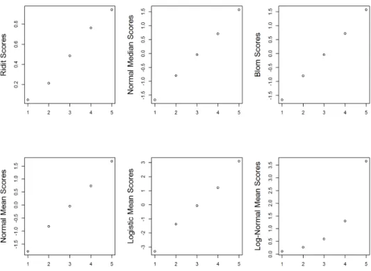
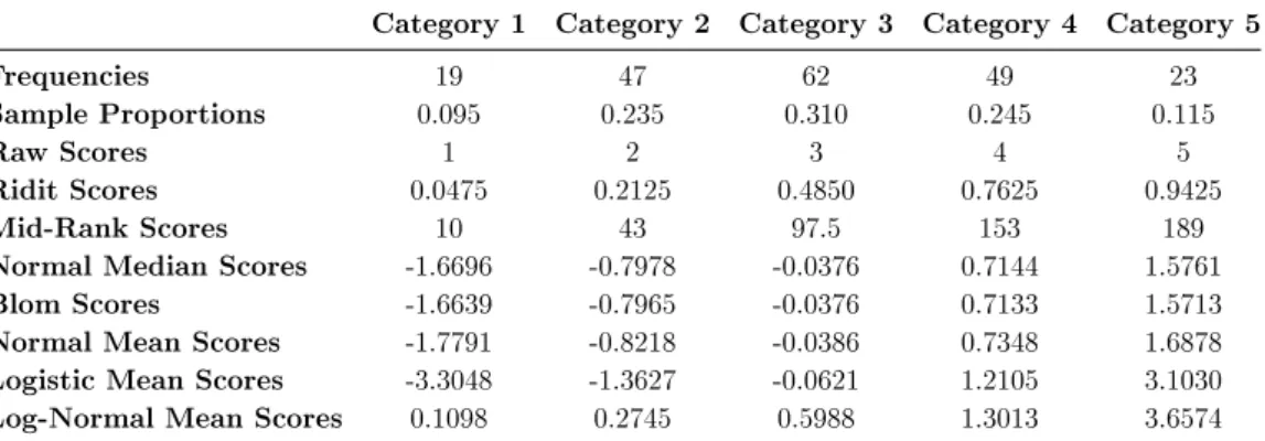
28 CHAPTER 2. SCORING METHODS To better understand the dierences between score types we also present in Figure 2.1 a graphical comparison of raw scores (on the abscissa axis) with the other methods of scoring. The reference ordinal variable has been generated, as for the computational times, randomly sampling from a standard normal variable, which has been subsequently discretized, considering ve categories (more details on the method used in order to generate ordinal variables will be provided in chapter 5). The scores have been computed on a sample of 200 observations.

We do not include in the graphs the comparison with mid-ranks as they are just a linear transformation of ridits, so the relative distances between categories would be the same. Mid-ranks are included in the Table 2.4, where the sample proportions, together with the numeric values for the scores presented in the graphs are provided.

(50)

2.2. THE SCORING METHODS 29 As expected, we do not observe relevant dierences between normal median and blom scores from the graph in Figure 2.1 (dierences are at the third decimal place as it possible to see from Table 2.4). With regard to normal mean and logistic mean scores we have that the scores for the high order categories are more spread for the latter method. The exception is category 3 (i.e. the central category), where the scores are similar due to the fact that both the underlying distributions are centred at 0. This is because the logistic distribution has slightly longer tails compared to the normal distribution. The main dierence in the score's trend is observed for the log-normal mean scores. In this case the scores are closer for the low order categories and the distance increases for high order categories. When data are generated as in this example, by discretizing from a continuous standard normal variable, we may expect that, in a classication context, using log-normal mean scores would bring the worst result with respect to all other scores.

Table 2.4: Score's value for simulated standard normal data

Category 1 Category 2 Category 3 Category 4 Category 5

Frequencies 19 47 62 49 23

Sample Proportions 0.095 0.235 0.310 0.245 0.115

Raw Scores 1 2 3 4 5

Ridit Scores 0.0475 0.2125 0.4850 0.7625 0.9425

Mid-Rank Scores 10 43 97.5 153 189

Normal Median Scores -1.6696 -0.7978 -0.0376 0.7144 1.5761 Blom Scores -1.6639 -0.7965 -0.0376 0.7133 1.5713 Normal Mean Scores -1.7791 -0.8218 -0.0386 0.7348 1.6878 Logistic Mean Scores -3.3048 -1.3627 -0.0621 1.2105 3.1030 Log-Normal Mean Scores 0.1098 0.2745 0.5988 1.3013 3.6574

Again we remark that the location of the underlying curve is not of interest in this context as long as the relative dierences between categories stay the same. A justication for this come from the simple realization that any classi-er should be able to identify the best subdivision region among obsclassi-ervations into classes, regardless of translations of the data values (i.e. a reasonable classier should be invariant with respect to linear transformations). For ex-ample, suppose that we a