Stock Price Prediction using Adaptive Time Series Forecasting and Machine Learning Algorithms

(1)

UNIVERSITY OF CALIFORNIA Los Angeles

A thesis submitted in partial satisfaction

of the requirements for the degree Master of Applied Statistics

by Lumeng Chen

(2)

(3)

ABSTRACT OF THE THESIS

Stock Price Prediction using Adaptive Time Series Forecasting and Machine Learning Algorithms

by

Lumeng Chen

Master of Applied Statistics

University of California, Los Angeles, 2020

Professor Yingnian Wu, Chair

In this thesis, ARIMA model, Long Short Term Memory (LSTM) model and Extreme Gradient Boosting (XGBoost) models were developed to predict daily adjusted close price of selected stocks from January 3, 2017 to April 24, 2020. Daily stock price data includes columns of open, close, adjusted close, high, low and volume. In ARIMA and LSTM models, the only features we used as model inputs were p e io N da ock p ice . P edic ion on da N+1 a calc la ed ba ed on

previous N values. RMSE and MAPE were calculated from this rolling forecast and the actual price in the test dataset. Optimal parameters were selected to be the setting that yielded the lowest RMSE score. Residuals diagnostic was performed to check model assumption for the final ARIMA model. In XGBoost model, feature engineering was used to create two additional features from open, close, high and low price. Same with LSTM model, previous N days features were used as

(4)

features in day N+1 for prediction. In both LSTM and XGBoost models, training dataset was scaled for model fitting. Features and output from cross-validation and test dataset were scaled too

ba ed on p e io N da al e . The p edic ion e l were then reverted back to original scale before calculation of RMSE and MAPE scores.

In conclusion, looking at the prediction versus actual stock price plot for each stock and their RMSE and MAPE scores, all three models produced good fo eca of ne da stock price. However, during the time with great volatility, the lag between forecast value and actual value is more noticeable. In our models, historical N days stock price on its own could provide a relatively

acc a e p edic ion on N+1 da ock p ice. In XGBoost model particularly, we found out that N=2 provided better RMSE and MAPE(%) results than other larger values of N (previous N days). As N gets larger, prediction accuracy got lower in XGBoost. In XGBoost feature importance analysis, the most impo an fac o o oda ock p ice i i p ice e e da . Although the final ARIMA model achieved the lowest RMSE score, grid search for one-step ARIMA forecast model parameters took the longest computing time, while XGBoost model with the second lowest RMSE score required the least time for parameter tuning and forecast calculation.

(5)

The thesis of Lumeng Chen is approved.

Frederic R. Paik Schoenberg Nicolas Christou

Yingnian Wu, Committee Chair

University of California, Los Angeles 2020

(6)

List of Tables

Table 1 VTI stock price data ... 3

Table 2 Training and test dataset split ... 3

Table 3 Data summary of VTI, AMZN, MSFT and GOOG ... 6

Table 4 Ljung-Box Test ... 18

Table 5 ARIMA model results for MSFT, GOOG and AMZN ... 18

Table 6 Tuning optimizer... 24

Table 7 LSTM parameters after tuning ... 25

Table 8 LSTM model results for MSFT, GOOG and AMZN ... 26

Table 9 RMSE and MAPE (%) for N ... 30

Table 10 VTI training data ... 31

Table 11 XGBoost parameters after tuning ... 35

Table 12 XGBoost model results for MSFT, GOOG and AMZN ... 36

Table 13 Model Comparison ... 36

Table 14 ARIMA model Grid search RMSE and MAPE results ... 41

Table 15 SARIMA(p, d, q) x (P, D, Q, S) grid search output ... 43

Table 16 Tuning N in LSTM; Tuning epochs and batch_size in LSTM; Tuning LSTM_units and dropout_prob ... 44

Table 17 Tuning n_estimators and max_depth; Tuning learning_rate and min_child_weight .... 46

Table 18 Tuning subsample and gamma parameter; Tuning colsample_bytree and colsample_bylevel ... 47

(9)

List of Figures

Figure 1 Correlation plot ... 6

Figure 2 Stock price trend charts ... 7

Figure 3 VTI adjusted close price autocorrelation lag plot and distribution plot ... 9

Figure 4 VTI stock price forecast using ARIMA ... 13

Figure 5 Residuals plot ... 14

Figure 6 ACF and PACF of residuals ... 14

Figure 7 VTI stock price forecast using SARIMA(1, 1, 1) x (0, 1, 1, 30) ... 16

Figure 8 Standard RNN repeating module with single layer [5] ... 19

Figure 9 LSTM repeating module with interacting layers [5] ... 19

Figure 10 LSTM model flowchart ... 20

Figure 11 RMSE/MAPE(%) with N ... 22

Figure 12 Tuning epochs and batch_size ... 23

Figure 13 Tuning LSTM units and dropout probability ... 24

Figure 14 VTI stock price prediction on LSTM test dataset ... 25

Figure 15 VTI price without scaling and training series with scaling ... 31

Figure 16 Tuning n_estimators and max_depth... 32

Figure 17 Tuning subsample and gamma parameters... 33

Figure 18 Tuning colsample_bytree and colsample_bylevel ... 34

Figure 19 VTI stock price prediction on XGBoost test dataset ... 35

Figure 20 Time Series Decomposition of VTI train data ... 39

Figure 21 MSFT stock price forecast using ARIMA... 39

(10)

Figure 23 AMZN stock price forecast using ARIMA ... 40

Figure 24 MSFT stock price forecast using LSTM ... 47

Figure 25 AMZN stock price forecast using LSTM ... 48

Figure 26 GOOG stock price forecast using LSTM ... 48

Figure 27 MSFT stock price forecast using XGBoost ... 49

Figure 28 GOOG stock price forecast using XGBoost ... 49

Figure 29 AMZN stock price forecast using XGBoost ... 50

(11)

1. Introduction

1.1 Introduction and Outline

Machine learning algorithms are known to be very effective in prediction problems. One of its application is predicting time series. In this paper, we applied a few adaptive models, XGBoost, LSTM and ARIMA models to predict stock price of Vanguard Total Stock Market ETF (ticker: VTI), Amazon (ticker: AMZN), Microsoft (ticker: MSFT) and Google (ticker: GOOG). Predicting stock price with 100% accuracy is almost impossible in reality as stock price is heavily influenced by unquantifiable factors, such as market irrational behavior and news. In this thesis, forecast model fitting and parameter tuning for VTI adjusted close price is discussed in detail as an example. For other stocks, we applied the same model development procedure as illustrated in VTI and compared their prediction results to see if model performance is consistent across different stocks. Unlike other models where trading volume, opening price and other technical indicators are fed into the model, we built our ARIMA and LSTM models only use adjusted close price in previous N days as input to predict price on day N+1. This is because although stock price might be affected by other factors, it is largely dependent on historical stock price. In XGBoost model, difference between high and low price; difference between open and close price and volume were added as features to the model through feature engineering. All features from previous N days were added as features to predict stock price on N+1 day too.

In chapter 1, we briefly introduced selected stock portfolio and the performance metrics chosen for model fo eca pe fo mance comparison. In chapter 2, data summary of stock data of VTI, MSFT, GOOG and AMZN was reviewed. We found out that they are highly correlated but with significantly different volatility (standard deviation).In the following chapters, we investigated if model prediction performance for each method can remain consistent across various stocks. In

(12)

chapter 3, ARIMA rolling forecast model was built on the training dataset of VTI stock price time series and grid search for optimal parameter settings was performed. RMSE score was calculated to find the optimal parameter setting. Residuals diagnostic was conducted to check model assumption. Seasonal ARIMA (SARIMA) one-step forecast model was also examined to see if it has better prediction accuracy based on RMSE score. Grid search of SARIMA model parameters was performed too and the optimal parameter setting was selected based on AIC. With the same process, ARIMA models have been developed for the other three stocks. RMSE and MAPE (%) were calculated for model comparison. In chapter 4 and chapter 5, we went through LSTM and XGBoost model methodology respectively. Original parameters were used to develop model on training dataset of VTI stock price. Model parameters were tuned on development dataset and model prediction performance was assessed on test dataset. The same process was performed for the other stocks data. In chapter 6, prediction metrics were compared and discussion has been made for LSTM, ARIMA and XGBoost models. Future potential research topic for stock price forecasting was mentioned.

1.2 Data Description

Four ock data, Amazon (ticker: AMZN), Microsoft (ticker: MSFT), Vanguard Total Stock Market ETF (ticker: VTI) and Google (ticker: GOOG), are collected from Yahoo! Finance. Each dataset has attributes of open, high, low, closing, adjusted closing price and trading volume as shown below.

(13)

Table 1VTI stock price data

For all stock indices, daily adjusted closing price is used as response variable in each model. Adjusted closing price is obtained by factoring in any factor, for example, corporate actions such as stock splits, dividends or distributions, which might affect the stock price to the closing price after the market closes. It is considered to be the true price of a stock and is often used when examining historical returns or performing a detailed analysis historical return. For model prediction, we are only interested in forecasting adjusted closing price for simplicity and consistency. It is understood that model comparison results should hold if we chose other types of price as dependent variable for the same index. When building Extreme Gradient Boosting (XGBoost) model, all other data points, open, close, high, low prices and trading volume were used too as input for the model. For other models, only daily adjusted closing price from previous days with different lags were fed into the model to determine the optimal parameter setting.

LSTM and XGBoost

Period Start End Length

Training Jan-17 Dec-18 501

Cross-validation Jan-19 Aug-19 166

Test Sep-19 Apr-20 166

ARIMA

Period Start End Length

Training Jan-17 Aug-19 666

Test Sep-19 Apr-20 167

(14)

In terms of time period selection, January 3, 2017 to April 24, 2020 is selected for training and test datasets for all models with the split shown in table 2. In total, there are 833 observations in the dataset. For Long Short Term Memory model (LSTM) and XGBoost models, split for training, cross-validation (development) and test dataset are 60%, 20% and 20% respectively.

Cross-alida ion da a e i c ea ed o ne model h pe pa ame e . In ARIMA model development, 80% of the data is used for training dataset and 20% is for test dataset. Number of observations in each dataset is listed in table 2 above. Models were trained on the training set and model performance were reported on the test dataset.

1.3 Comparison Metrics RMSE and MAPE

Root Mean Square Error (RMSE) and Mean Absolute Percentage Error (MAPE) are statistical measure of how accurate a forecast model is. RMSE is used to measure difference between actual values and forecasted in the test dataset. It represents the square root of the second sample moment of the differences between predicted values and observed values. RMSE aggregates the magnitudes of the errors in predictions across various time periods into a single measure of predictive power by taking the average of the error by number of fitted points. RMSE is a measure of accuracy, to compare forecasting errors of different models for the same dataset as it is scale-dependent. RMSE is calculated as follows:

RMSE =

∑nt=1(Ft−At)2 n

MAPE measures prediction accuracy of a forecast model. It is calculated by summing the ratio of difference between actual value and forecasted value over actual value, then take the average of

(15)

this sum by the number of fitted points n. It usually expresses the accuracy as a ratio defined by formula: MAPE = 1 𝑛

∑

|

−

|

𝑛 =1

,

where At is the actual value and Ft is the forecast value. Sometimes, because MAPE takes division of error by the actual value individually, it has the risk of being too skewed. A big error with a low

ac al al e ha a h ge impac on MAPE. D e o hi , model pa ame e ning was based on RMSE score, as optimizing MAPE may result in an inaccurate forecast which is most likely to undershoot the actual value.

2. Descriptive Time Series Analysis

2.1 Descriptive Data Analysis

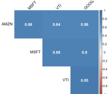
Below figure 2 demonstrated trends of selected stocks during selected time frame. MSFT, GOOG and AMZN has similar trend with VTI, however, AMZN and GOOG has much greater price range than MSFT and VTI. AMZN adj ed clo ing p ice anged f om $1,000 from the beginning of 2017 to currently around $2,500, hile VTI and MSFT p ice ange are historically under $200. Additionally, as can be seen from correlation plot (figure 1), all four stocks are highly correlated with each other with correlation coefficient higher than 0.80. This is because MSFT, GOOG and AMZN share the similar growth trends as they are all technology companies with similar characteristics. In addition, MSFT, AMZN and GOOG make up 4.77%, 3.26% and 1.35% respectively of the VTI portfolio1. It is reasonable for them to have such high correlation. However,

as can be seen from table 3, GOOG and MSFT have much higher volatility (standard deviation) [18] [

(16)

than MSFT and VTI while VTI has the lowest volatility. Whether or not our forecasting models share the similar forecasting performance for all stocks are investigated in later chapters.

VTI AMZN MSFT GOOG

count 833 833 833 833 mean 135.48 1,516.50 105.15 1,098.57 std 14.22 400.37 32.34 154.99 min 109.30 753.67 58.87 786.14 25% 124.49 1,100.95 78.82 992.81 50% 135.67 1,643.24 102.77 1,102.23 75% 144.96 1,823.29 133.16 1,194.43 max 171.32 2,410.22 188.19 1,526.69

Table 3Data summary of VTI, AMZN, MSFT and GOOG

Figure 1 Correlation plot

(17)

Figure 2 Stock price trend charts

3. ARIMA Model

3.1 Methodology

ARIMA stands for Auto-Regressive Integrated Moving Averages. ARIMA(p, d, q) is a generalization of an autoregressive moving average (ARMA(p, q)) model. ARIMA models are applied in some cases where data show evidence of non-stationarity. The AR term p of ARIMA

(18)

indicates that the evolving variable of interest is regressed on its own lagged (i.e., prior) values. For example, if p is 3, the predictors for yt will be yt−1, … , yt− . The MA part indicates that the regression error is actually a linear combination of error terms whose values occurred contemporaneously and at various times in the past. For example, if q is 5, the predictors for y_t will include t−1, … , yt− . The I (for "integrated") indicates that the data values have been replaced with the difference between their values and the previous values (and this differencing process may have been performed more than once) [1]. Generalized ARMA(p, q) process is defined as below [1]:

E( t, s) = 0, for t s

y_t = μ + a_ty_t−1+ ⋯ + a y_t− + _t+ b_{1 t−1}+ ⋯ + b _t−

Where ai are the parameters of the autoregressive part of the model and bi are the parameters of the moving average part and _i are the error terms.

As a simplified notation, this is often expressed in terms of lag-polynomials as Φ(L)y_t = ψ(L) _t

Where

Φ(L) = 1 − a₁L1− a₂L2− ⋯ − a L ψ(L) = 1 + b₁L1_{+ b}

2L2+ ⋯ b L L is the lag or shift operator, Lix_t = x_t−i, L0 = 1. [1]

Seasonal Arima (SARIMA) model was also examined to see if it can provide better prediction for stock price. SARIMA(p, d, q)(P, D, Q, S) includes non-seasonal orders: p for autoregressive order; d for differencing order and q for moving average order. (P, D, Q, S) is seasonal orders: P for seasonal autoregressive order; D for seasonal differencing order; Q for seasonal moving average

[1] [1] [1]

(19)

order and S is number of time steps per cycle [17], in other words, the specified periodicity of time series.

3.2 ARIMA model fitting of VTI stock price

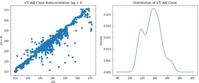
Figure 3 VTI adjusted close price autocorrelation lag plot and distribution plot

As can be observed from figure 3, autocorrelation lag plot of VTI adjusted close price closely follows a straight line. Its distribution looks normal. Both plots suggest that ARIMA would be a good model for the data.

VTI adjusted close price series was split into 80% training data and 20% test data. One-step forecast was preformed over the test dataset. We used training dataset to fit the model and generate a prediction for each day in the test dataset. A rolling forecast was performed given the dependence on observations in prior time steps. An ARIMA model was recreated after each new observation is received to generate the rolling forecast. All observations are manually tracked and stored in a list called history that is seeded with the training data and to which new observations are appended

(20)

each iteration. Below is the code we used to generate rolling forecast from ARIMA model and calculate MAPE and RMSE score on test dataset [19]:

train_ar = train_data['adj_close'].values test_ar = test_data['adj_close'].values

history = [x for x in train_ar] print(type(history))

predictions = list()

for t in range(len(test_ar)):

model = ARIMA(history, order=(8,0,1)) model_fit = model.fit(disp=0) output = model_fit.forecast() yhat = output[0] predictions.append(yhat) obs = test_ar[t] history.append(obs)

error = math.sqrt(mean_squared_error(test_ar, predictions)) print('Residual Mean Squared Error: %.3f' % error)

error2 = mape_fun(test_ar, predictions)*100

print('mean absolute percentage error: %.3f' % error2)

3.3 Tuning p, d, q

Grid search for optimal (p, d, q) setting was performed on training dataset. RMSE and MAPE scores were calculated from prediction on the test dataset and the actual value in test dataset. The

(21)

(p, d, q) combination yielded lowest RMSE was selected as final ARIMA model using code [20] below:

# evaluate an ARIMA model for a given order (p,d,q)

def evaluate_arima_model(X, arima_order):

train_size = int(len(X) * 0.8) # prepare training dataset train, test = X[0:train_size], X[train_size:]

history = [x for x in train] predictions = list() for t in range(len(test)):

model = ARIMA(history, order=arima_order) model_fit = model.fit(disp=0)

yhat = model_fit.forecast()[0] predictions.append(yhat) history.append(test[t])

rmse = math.sqrt(mean_squared_error(test, predictions)) # calculate out of sample error return rmse

# evaluate combinations of p, d and q values for an ARIMA model

def evaluate_models(dataset, p_values, d_values, q_values): dataset = dataset.astype('float32')

best_score, best_cfg = float("inf"), None

for p in p_values: for d in d_values: for q in q_values: order = (p,d,q) try:

(22)

rmse = evaluate_arima_model(dataset, order) if rmse < best_score:

best_score, best_cfg = rmse, order

print('ARIMA%s RMSE=%.3f' % (order,rmse)) except:

continue

print('Best ARIMA%s RMSE=%.3f' % (best_cfg, best_score)) # evaluate parameters

p_values = [0, 1, 2, 4, 6, 8] d_values = range(0, 3) q_values = range(0, 3)

evaluate_models(df['adj_close'].values, p_values, d_values, q_values)

Residual Mean Squared Error: 2.985 Mean Absolute Percentage Error: 9.675

As can be seen from logic above, p value was selected from 0, 1, 2, 4, 6, 8 and ranges for d and q values were from 0 to 3. Grid search results are provided in table 14 in Appendix A. In the output results, RMSE for ARIMA models ranged from 2.985 to 22.457 and MAPE ranged from 9.513% to 12.457%. ARIMA (8, 0, 1) produced the lowest RMSE of 2.985 with 9.675% MAPE, while the lowest MAPE was produced by ARIMA (0, 0, 1) with 11.978 RMSE. In comparison, one-step forecast model, ARIMA(8, 0, 1), has the lowest value in RMSE and relatively low MAPE metrics. Therefore, ARIMA(8, 0, 1) was selected as forecast model for VTI stock price and the next step is to check residuals diagnostics.

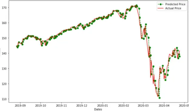
As can be seen from figure 4, one-step forecast using ARIMA model provided accurate predictions

(23)

beginning of 2020. MAPE score of approximately 9.675% indicates the model is approximately 90.325% accurate in predicting test set observations.

Figure 4 VTI stock price forecast using ARIMA

3.4 ARMA(8,0,1) Model Diagnostic

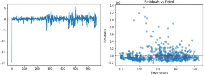
As can be observed from figure 5 below, the residuals versus order plot (left) indicates that the residuals did not violate the assumption of constant location and scale. Residuals appeared to be random with most of points scattered in the range of (-1, 1). From residuals versus fitted plot on the right, we can see that the most of residual points fall randomly on both sides of 0, with no recognizable patterns in the points. The fitted red line is also a relatively flat line. Based on the plot, it is reasonable to conclude that residuals are unbiased and have a constant variance. Therefore, the forecast is accurate.

(24)

Figure 5 Residuals plot

Autocorrelation and partial autocorrelation plots for residuals are also reviewed below. The autocorrelation function is a measure of the correlation between the observations of a time series that are separated by k time units. The partial autocorrelation function is a measure of the correlation between the observations of a time series that are separated by k time units (y_tand yt− ), after adjusting for the presence of all the other terms of shorter lag (yt−1, yt−2, ... , yt− −1) [16]. From below autocorrelation and partial correlation plot, since there are no significant correlations present (correlation lags exceed the blue shaded confidence interval), we can conclude that model meets assumption and the residuals are independent. Ljung-box test will be used later

o check e id al andomne again la e .

(25)

3.5 Comparison with SARIMA model

Since seasonality was not considered in above ARIMA model, here we checked if including

seasonal parameter could fit the training data better, in other words, check if the series has seasonality. SARIMA(p, d, q) x (P, D, Q, S) model which models seasonal effect in a multiplicative way is used. We used a g id ea ch o i e a i el e plo e diffe en combina ion of pa ame e .

For each combination of parameters, we fitted a new seasonal ARIMA model with the SARIMAX() function from the statsmodels module [3] and assess its overall quality. P and q were set to iterate between 0 and 2 as shown below [14]:

for param in pdq:

for param_seasonal in seasonal_pdq: try: mod = sm.tsa.statespace.SARIMAX(train_ar, order=param, seasonal_order=param_seasonal, enforce_stationarity=False, enforce_invertibility=False) results = mod.fit()

print('ARIMA{}x{}30 - AIC:{}'.format(param, param_seasonal, results.aic)) except:

continue

with example output as follows:

ARIMA(0, 0, 1)x(0, 1, 0, 30)30 – AIC: 3271.08542290716 ARIMA(0, 0, 1)x(0, 1, 1, 30)30 - AIC: 3128.19644907746

(26)

Different combinations of SARIMA(p, d, q) x (P, D, Q, S) were produced. Within those models, Akaike information criterion (AIC) was used to select the optimal SARIMA model. AIC estimates the relative amount of information lost by a given model: the less information a model loses, the higher the quality of that model. All generated seasonal ARIMA model is provided in table 15 in Appendix. SARIMA model with parameter (1, 1, 1) x (0, 1, 1, 30) has the lowest AIC and was selected as optimal SARIMA model.

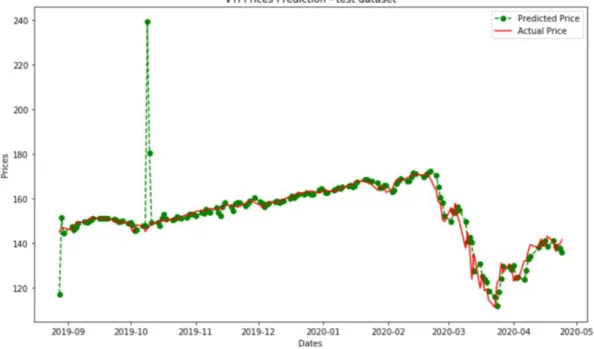
One-step-ahead prediction was calculated and RMSE for this model is 8.538. From below prediction plot under SARIMA model we can see that there are a few significant outliers in predictions. Also, seasonality in the predictions of test dataset are exaggerated since green dotted line fluctuates more notably than red line of actual values. This may give rise to the higher RMSE score. As RMSE of one-step forecast SARIMA model was much greater than RMSE of rolling forecast ARIMA(8, 0, 1) model, ARIMA(8, 0, 1) was selected as optimal model for VTI stock price forecast.

(27)

3.6 Ljung Box Test

The Ljung Box test (named for Greta M. Ljung and George E. P. Box) is a type of statistical test of whether any of a group of autocorrelations of a time series are different from zero. Instead of testing randomness at each distinct lag, it tests the "overall" randomness based on a number of lags [4]. It is closely connected to Box-Pierce test.

The null hypothesis of the Ljung-Box Test, 𝐻₀, is that the data are independently distributed (i.e. the correlations in the population from which the sample is taken are 0, so that any observed correlations in the data result from randomness of the sampling process). In other words, the data is white noise. The alternative hypothesis, 𝐻 , is that the data are not independently distributed; they exhibit serial correlation [4].

The Ljung-Box test is commonly used in ARIMA modeling. It was applied to the residuals of our fitted ARIMA model to test if residuals from the model have no autocorrelation. From below Ljung-Box test results table we can see that for first 40 lags, p-values are greater than 0.05, indicating residuals are randomly distributed and there is no autocorrelation existed in the residuals. Assuming lags exceeding 40 lags exhibited the same pattern, it is safe to say that the model provided an adequate fit to the data.

lb_stat lb_pvalue lb_stat lb_pvalue 1 0.14528 0.703088 21 12.927604 0.911139 2 0.154784 0.925527 22 12.941089 0.934791 3 0.21824 0.974592 23 13.017169 0.951617 4 0.252353 0.992679 24 14.585595 0.932301 5 0.253394 0.998429 25 14.680218 0.948541 6 0.321333 0.999387 26 14.970633 0.957869 7 0.33805 0.99985 27 15.272168 0.965439 8 0.650867 0.999639 28 15.935448 0.966766 9 0.670169 0.999894 29 16.690533 0.966772

(28)

10 0.67341 0.999973 30 16.764278 0.975295 11 0.696224 0.999992 31 17.752599 0.972579 12 0.699729 0.999998 32 17.833207 0.97954 13 0.726276 0.999999 33 17.870176 0.985186 14 4.991091 0.985936 34 18.007931 0.988851 15 5.549907 0.986358 35 18.058528 0.992028 16 6.282142 0.984751 36 18.201858 0.99407 17 9.793694 0.912038 37 19.528586 0.991877 18 10.453063 0.91611 38 19.561854 0.994236 19 10.884056 0.927677 39 19.585032 0.995973 20 12.859491 0.883331 40 20.09682 0.996361

Table 4Ljung-Box Test

3.7 Model Fitting for MSFT, GOOG and AMZN

Table 5 below shows ARIMA model fitted for MSFT, GOOG and AMZN with their respective MAPE and RMSE scores for comparison with other models. MSFT, GOOG and AMZN stock price forecast plots are included in Appendix A as figure 21-23.

ARIMA Model RMSE MAPE MSFT (8, 1, 1) 3.985 10.700% GOOG (8, 1, 1) 26.974 9.714% AMZN (8, 1, 1) 38.069 8.161%

Table 5ARIMA model results for MSFT, GOOG and AMZN

4. Long Short Term Memory Model

4.1 Methodology

LSTM model is a special kind of Recurrent Neural Network (RNN) and was developed to combat the vanishing gradients problem in training traditional RNNs. Unlike standard feedforward neural networks, LSTM has feedback connections which is capable of learning long-term dependencies. LSTM has three gates: the input gate, the forget gate and the output gate. The update gate adds

(29)

information to the cell state. The forget date determines and removes information that is no longer required by the model. The output gate determines the amount of information to output as activations to the next layer. LSTM is introduced by Hochreiter & Schmidhuber (1997). Compared with standard RNN, which has a simple structure with a single tanh layer (figure 8),

Figure 8Standard RNN repeating module with single layer [5]

LSTM has four interacting layers in each repeating module in the same chain-like structure (figure 9). In the figure 9, each line carries an entire vector, from the output of one node to the inputs of others. The pink circles represent pointwise operations, like vector addition, while the yellow boxes are learned neural network layers. Lines merging denote concatenation, while a line forking denotes its content being copied and the copies going to different locations [5].

(30)

The first step in LSTM is to decide what information would be forgotten from the cell state. This

deci ion i made b a igmoid la e called fo ge ga e la e . It looks at ht−1 and xt, and outputs a number between 0 and 1 for each input from cell state C_t−1, he e 1 ep e en comple el keep hi hile a 0 ep e en comple el ge id of hi . C_t−1 is then updated into the new cell state C_t. This process is represented by below formulae [5]:

i_t = σ(W_i· [h_t−1, x_t + b_i C_t = tanh(W_C∙ [h_t−1, x_t + b_C)

The old state is then multiplied by f_t, forgetting the things we decided to forget earlier, then we add new candidate values scales by how much we decided to update each state value, i_t∙ C_t.

C_t = f_t∙ C_t−1+ i_t∙ C_t

Finally, we run a sigmoid layer which decides what parts of the cell state we are going to output. Then we put the cell state through tanh, which outputs value between -1 and 1, and multiply it by the output of the sigmoid gate, so that we only output the parts we decided to.

o_t = σ(W_o∙ [h_t−1, x_t + b_o h_t = o_t∙ tanh (C_t)

In our adjusted close price forecast model, we use two layers of LSTM modules, and a dropout layer in-between to avoid over-fitting as shown in figure 10.

Figure 10LSTM model flowchart

[5]

(31)

4.2 Model Fitting of VTI stock price

Keras API from TensorFlow package of Python is used to build LSTM model for VTI adjusted close price data, VTI price data was split into 80% training data, 20% cross-validation data and 20% test data. Training dataset was scaled so that each data point has mean zero and standard deviation one. In the scaled training set, we started building LSTM model with initial setting to use past 9 da a fea e fo p edic ion of oda al e. Given that there are 501 observations in the training dataset, the scaled training input and outcome variables has length of 492 and timespan of 9. Cross-validation and test dataset each has length of 166. Train dataset was scaled to have mean zero and standard deviation of one. For each prediction on the development and test dataset, previous N day values, used for features and output, were scaled to have mean 0 and 1. The prediction results were reverted back to original scale by multiplying the previous N day standard deviation and adding back the previous N days mean. RMSE and MAPE scores were calculated between prediction results and the actual stock price at day N.

Initial settings for other LSTM parameters are as follows: dropout probability of 1; LSTM_Units of 50, where LSTM_units is the number of hidden units pertinent to the length of state vector,

hich i al o called la en dimen ion [6]; Op imi e of Adam , hich i efe ing o Adam

algorithm, a stochastic descent method that is based on adaptive estimation of first-order and second-order moments [7]; epochs of 1 and batch size of 1. After running LSTM model with initial setting on development dataset, we obtained RMSE of 1.985 and MAPE of 1.149% for VTI adjusted close price prediction.

4.3 Parameter Tuning

(32)

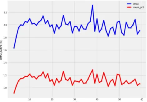
N in the range of 3 to 60 days were fed into LSTM model to find the optimal N which gives lowest RMSE and MAPE on the development dataset. As we can see from figure 11 below, blue line is RMSE score and red line is MAPE (%), optimal N =3 is obtained with lowest RMSE of 1.635 and lowest MAPE of 0.915%. (Table 4.1 of RMSE and MAPE results with different N is listed in Appendix A.)

Figure 11RMSE/MAPE(%) with N

2. Tuning epochs and batch_size

Epochs can be selected from [1, 10, 20, 30, 40, 50] and optimal value for batch_size can be selected from [8, 16, 32, 64, 128]. We ran LSTM model on development dataset to come up with the optimal parameter setting for epochs and batch_size based on RMSE and MAPE (%). As can be observed from figure 12 below, batch_size 8 (the blue line) with epochs of 50 produced the lowest RMSE of 1.247 and lowest MAPE (%) of 0.665%. (Table 4.2 of RMSE and MAPE results with different epochs and batch_size combinations are shown in Appendix A.)

(33)

Figure 12Tuning epochs and batch_size

1. Tuning LSTM units and dropout probability

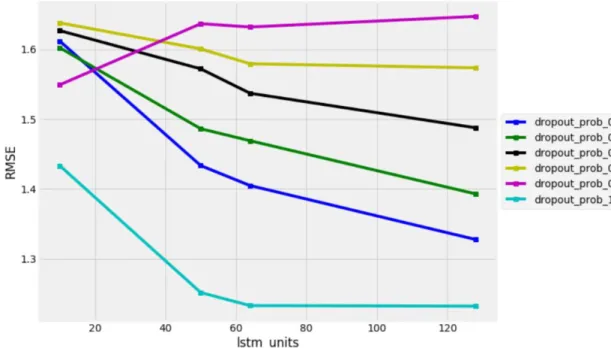
Optimal LSTM units and dropout probability were selected from [10, 50, 64, 128] and [0.5, 0.6, 0.7, 0.8, 0.9, 1] respectively on the development dataset. As can be observed from figure 13 below, dropout_prob of 1 (the blue line) with LSTM_units of 128 produced the lowest RMSE of 1.232

and lo e MAPE (%) of 0.644%. RMSE dec ea ing a e lo ed do n f om l m_ ni of 80

with dropout_prob of 1. (Table 4.3 of RMSE and MAPE results with different LSTM units and dropout probability combinations is shown in Appendix A.)

(34)

Figure 13Tuning LSTM units and dropout probability

2. Tuning optimizer

Optimal optimizer was selected from ['adam', 'sgd', 'rmsprop', 'adagrad', 'adadelta', 'adamax', 'nadam'] on the development dataset. As can be observed from table 6 below, adamax produced the lowest RMSE of 1.233 and MAPE (%) of 0.651%.

optimizer rmse mape_pct

adam 1.235473 0.648086 sgd 1.567141 0.875689 rmsprop 1.233444 0.644605 adagrad 1.27349 0.68625 adadelta 1.240973 0.656432 adamax 1.233297 0.650866 nadam 1.237552 0.644601

(35)

4.4 Final Model and Prediction results

After tuning, below optimal parameters (table 7) were selected to replace original parameter setting on development dataset. LSTM model was then applied to test dataset. RMSE on test dataset is 3.227 while MAPE on test dataset is 1.336%. As can be observed from figure 14, LSTM was able to predict VTI price more accurately when it is less volatile. There is almost no visual lag before February 2020, but we can see a slight lag in predictions on the plot after February 2020.

param original after_tuning

N 9 3

lstm_units 50 128

dropout_prob 1 1

optimizer adam adamax

epochs 1 50

batch_size 1 8

rmse 1.98851 1.23946

mape_pct 1.14488 0.6445 Table 7LSTM parameters after tuning

(36)

4.5 Model fitting for MSFT, AMZN and GOOG

Table 8 below shows LSTM model fitted for MSFT, GOOG and AMZN with their respective MAPE and RMSE scores. MSFT, GOOG and AMZN stock price forecast price under LSTM are included in Appendix A as figure 24-26.

LSTM RMSE MAPE

MSFT 4.278 1.699%

GOOG 29.263 1.525%

AMZN 43.585 1.509%

Table 8 LSTM model results for MSFT, GOOG and AMZN

5. Extreme Gradient Boosting Model

5.1 Methodology

XGBoo and fo E eme G adien Boo ing , he e he e m G adien Boo ing originates from the paper Greedy Function Approximation: A Gradient Boosting Machine, by Friedman [8]. Gradient boosting is a process to convert weak learners to strong learners, in an iterative fashion. According o F iedman g adien boo ing algo i hm [8], on each iteration, the gradient descent is first computed in order to fit a new base learner function. Once the best gradient descent step direction and size are found, the function estimation is updated. Gradient boosting is an approach where new models are created that predict the residuals or errors of prior models and then added together to make the final prediction. It is called gradient boosting because it uses a gradient descent algorithm to minimize the loss when adding new models [11]. In pseudocode, the generic gradient boosting method is [8][12]:

Input: training set {(x_i, y_i)}_i=12 _{a differentiable loss function}_{L(y, F(x))}_{, number of iterations M.} Algorithm:

(37)

1. Initialize model with a constant value: F₀(x) = argminγ∑ni=1L(yi, γ). 2. For m=1 to M:

1. Compute so-called pseudo-residuals: for 𝑖 = 1, . . . , 𝑛,

r_im = − ∂L(yi, F(xi))

∂F(x_i) , where F(x) = Fm−1(x)

2. Fit a base learner (or weak learner, e.g. tree) 𝑔 (𝑥) to pseudo-residuals, i.e. train it using training set {(x_i, r_im)}_i=1n _.

3. Compute multiplier 𝛾 by solving the following one-dimensional optimization problem:

γ_m= argmin_γ∑ L(y_i, F_m−1(x_i) + γg_m(x_i)) n

i=1

4. Update model: F_m(x) = F_m−1(x) + γ_mg_m(x) 3. Output FM(x).

XGBoost is an implementation of gradient boosted decision trees algorithm designed for computational speed and model performance, developed by Tianqi Chen [9]. It supports three main gradient boosting methods: gradient boosting machine (GBM) including the learning rate; Stochastic gradient boosting which is the boosting with sub sampling at the row, column and column per split levels; and regularized gradient boosting with L1 or L2 regularization [11]. Different with from GBM which divides the optimization problem into two parts by first determining the direction of the step and then optimizing the step length, XGBoost tries to determine the step directly by solving below equation for each x in the dataset [13]

∂L(y, fm−1(x) + f_m(x)) ∂fm(x)

(38)

By taking second-order Taylor expansion of the loss function and the current estimate fm−1_(x)_, we get L(y, fm−1(x) + f_m(x)) ≈ L(y, fm−1_{(x)) + g}

m(x)fm(x) + 1

2hm(x)fm(x)

2_{, where}_g

m(x) is the gradient and ℎ (𝑥) is the Hessian at the current estimate: h_m(x) = ∂2L( ,f(x))

∂f(x)2 where f(x) =

fm−1(x). Then, loss function can be rewritten as

L(f_m) ≈ ∑[g_m(x_i)f_m(x_i) +1 2hm(xi)fm(xi) 2 _{+ const.} n i=1 ∝ ∑ ∑ [g_m(xi)wjm+ 1 2hm(xi)wjm 2 i∈ _jm Tm j=0

Letting G_jmrepresents the sum of gradient in region j and H_jm equals to the sum of hessian in region j, the equation can be rewritten as L(f_m) ∝ ∑Tm[G_jmw_jm

j=1 +

1

2Hjmwjm

2 _{[13]. With the fixed}

learned structure, for each region, the optimal weight is w_jm = −Gjm

H_jm, j = 1, … , Tm. Therefore, the loss function is L(f_m) ∝ −1 2∑ G_jm2 H_jm Tm

j=1 [13]. According to Chen [9], this is structure score for a tree. The smaller the score is, the better the structure is. Thus, for each split made, the proxy gain is

defined as Gain =1 2[ G_jmL2 HjmL+ G_jm2 Hjm + G_jm2 Hjm = 1 2[ G_jmL2 HjmL+ G_jm2 Hjm − G_jmL+G_jm2 2 HjmL+Hjm [8][13].

Next step is to take regularization into consideration, the loss function becomes below:

L(f_m) ∝ ∑[G_jmw_jm T_m j=0 +1 2Hjmwjm 2 _{+ γT} m+ 1 2γ ∑ wjm 2 _{+ α ∑} _|w jm| T_m j=1 T_m j=1 = ∑[G_jmw_jm Tm j=0 +1 2(Hjm+ λ)wjm 2 _{+ α|w} jm| + γTm [13] [13]

(39)

Where γ is the penalization term on the number of terminal nodes, α and λ are for L1 and L2 regularization respectively. The optimal weight for each region j is defined as:

w_jm = { −Gjm+ α H_jm+ λ, Gjm < −α −Gjm− α Hjm+ λ , Gjm> α 0, else. The gain of each split is defined as [8][13]

Gain =1 2[ T_α(G_jmL)2 H_jmL+ λ + T_α(G_jm )2 H_jm + λ − T_α(G_jm)2 H_jm+ λ ] − λ, Tα(G) = { G + α, G < −α G − α, G > α 0, else

5.2 Model Development of VTI stock price

The XGBoost model was trained on the training dataset, its parameters were tuned in development dataset and we obtained prediction results on the test dataset. The same as previous LSTM model, VTI adjusted closing price of previous N days were used as features in the model to predict price on N+1 day. However, in this model, feature engineering has been performed and below 2 additional features were created:

1. range_hl: the range between high price and low price of the last N days. 2. range_oc: the range between open and close price of the last N days.

Training dataset has been scaled to have mean 0 and standard deviation 1 too. In addition, for development and test dataset, previous N da features, such as adjusted closing price, volume, range_hl etc., were all scaled to have mean 0 and standard deviation 1. It is worth noting here that instead of using the same scaling across training, development and test dataset, we used mean and variance of previous N days to scale features and predicted values in all datasets. Predictions were later reverted back to their original scale for output and calculation of RMSE and MAPE.

(40)

Initial model parameter setting is shown below, where n_estimators = 100 is number of boosted trees to fit; max_depth = 3 is maximum tree depth for base learners; learning_rate = 0.1 is boosting learning rate and min_child_weight = 1 is minimum sum of instance weight (hessian) needed in a child; gamma = 0 is minimum loss reduction required to make a further partition on a leaf node of a tree.

XGBRegressor(base_score=0.5, booster=None, colsample_bylevel=1, colsample_bynode=1, colsample_bytree=1, gamma=0, gpu_id=-1, importance_type='gain', interaction_constraints=None, learning_rate=0.1, max_delta_step=0, max_depth=3, min_child_weight=1, missing=nan,

monotone_constraints=None, n_estimators=100, n_jobs=0, num_parallel_tree=1,

objective='reg:squarederror', random_state=100, reg_alpha=0, reg_lambda=1, scale_pos_weight=1, seed=100, subsample=1, tree_method=None, validate_parameters=False, verbosity=None)

N = 2 is used as model input, which means that for features at day t, we use data from t-1 and t-2 as additional features to be added to the data frame. Below table 9 shows RMSE and MAPE (%) value of different N on the development dataset. N=2 has the lowest RMSE and MAPE score.

N RMSE MAPE 2 1.7523 0.743% 3 1.9542 0.818% 4 2.1785 0.915% 5 2.3740 0.994% 6 2.5735 1.063% 7 2.7357 1.118% 14 3.8686 1.603%

Table 9 RMSE and MAPE (%) for N

Training, development and test dataset were divided into 80% (length 501), 20% (length 166) and 20% (length 166). After feature engineering, additional column of range_hl and range_oc were added. In the next step, features from previous 2 days were used as features of day 3 as can be seen

(41)

from table 10, where lag_1 used previous day data and lag_2 used the day before previous day features. Therefore, we have 499 data points in training dataset.

date adj_close volume month range_hl range_oc

order_ day adj_close_ lag_1 1/5/17 109.91947 2604000 1 0.689994 0.089996 2 110.135796 1/6/17 110.26749 2317600 1 0.879998 -0.210006 3 109.919472 1/9/17 109.84421 2461400 1 0.400001 0.319999 4 110.267487 1/10/17 109.92886 2055300 1 0.739998 -0.110001 5 109.844208 1/11/17 110.2769 2751800 1 0.75 -0.329994 6 109.928856 range_hl

_lag_1 range_oc_lag_1 volume_lag_1 adj_close_lag_2 range_hl_lag_2 range_oc_lag_2 volume_lag_2 0.770004 -0.619995 3228700 109.29867 1.060005 -0.049995 2731600 0.689994 0.089996 2604000 110.1358 0.770004 -0.619995 3228700 0.879998 -0.210006 2317600 109.91947 0.689994 0.089996 2604000 0.400001 0.319999 2461400 110.26749 0.879998 -0.210006 2317600 0.739998 -0.110001 2055300 109.84421 0.400001 0.319999 2461400

Table 10 VTI training data

Scaling was performed on training, development and test dataset. Plot 15 below shows how the time series of VTI adjusted closing price compared with training series after scaling.

Figure 15VTI price without scaling and training series with scaling

As can be seen from output below, important features are dominated by adjusted_close price for the previous N days.

(42)

[('volume_lag_1', 0.0015100354), ('range_hl_lag_2', 0.0016028018), ('volume_lag_2', 0.0018247962), ('range_oc_lag_1', 0.0019524604), ('range_oc_lag_2', 0.0024724023), ('range_hl_lag_1', 0.0032888774), ('adj_close_lag_2', 0.40000784), ('adj_close_lag_1', 0.5873408)]

5.3 Parameter Tuning

1. Tuning n_estimators and max_depth

Candidates for number of estimators (fitted boosted trees) ranged from 10 to 250 with gap of 10. Maximum tree depth were selected from 2 to 9. As can be from seen from figure 16 below, max_depth of 2 with n_estimators of 20 achieved the lowest RMSE score. (Table 5.3 of detailed RMSE and MAPE(%) data for each combination of n_estimators and max_depth is provided in Appendix A.)

Figure 16Tuning n_estimators and max_depth

(43)

Candidates for optimal learning rate were 0.001, 0.005, 0.01, 0.05, 0.1, 0.2, 0.3. Minimum child weight can be selected from 5 to 20. Learning_rate of 0.1 and min_child_weight of 5 achieved the lowest RMSE score of 1.239. Table 5.4 of detailed RMSE and MAPE(%) data for each combination of learning_rate and min_child_weight is provided in Appendix A. As can be seen from table 5.4, learning rate is the main reason cause RMSE and MAPE (%) score to change. Various level of child weight does not change forecast accuracy notably for the same learning rate. 3. Tuning subsample and gamma parameters

Subsample ratio of the training instance can be selected from 0.1 to 1 and gamma can be selected from 0 to 0.8. Parameter setting of subsample = 0.1 and gamma = 0.3 (yellow line) yielded the lowest RMSE of 1.237, which can be seen from plot 18 below and table 5.5 in Appendix A.

Figure 17 Tuning subsample and gamma parameters

(44)

Colsample_bytree is the subsample ratio of columns when constructing each tree. Colsample_bylevel is the subsample ratio of columns for each split in each level. For both parameters, candidate values ranged from 0.5 to 1. As can be observed from plot 18, lowest RMSE of 1.237 was achieved with initial setting of colsample_bytree = 1 and colsample_bylevel = 1. (Table 5.6 with detailed information of RMSE and MAPE (%) scores for different combinations of colsample_bytree and colsample_bylevel is provided in Appendix A.)

Figure 18 Tuning colsample_bytree and colsample_bylevel

5.4 Final Model and Prediction results

After tuning, below optimal parameters (table 11) were selected on development dataset to replace original parameter setting. XGBoost model was ran on test dataset. RMSE on test dataset is 3.080 while MAPE on test dataset is 1.274%. This result is better than RMSE and MAPE (%) scores obtained in LSTM. As can be observed from prediction plot figure 19, XGBoo prediction of VTI price is quite accurate. Prediction produced by XGBoost is more accurately when it is less

(45)

volatile. There is almost no visual lag before February 2020, but we can see a slight lag in predictions on the plot after February 2020.

param original after_tuning

n_estimators 100 20 max_depth 3 2 learning_rate 0.1 0.1 min_child_weight 1 5 subsample 1 0.1 colsample_bytree 1 1 colsample_bylevel 1 1 gamma 0 0.3 rmse 1.249 1.237 mape_pct 0.665 0.650

Table 11 XGBoost parameters after tuning

(46)

5.5 Model Fitting for MSFT, AMZN and GOOG

Table 12 below shows XGBoost model fitted for MSFT, GOOG and AMZN with their respective MAPE and RMSE scores. MSFT, GOOG and AMZN stock price forecast price under XGBoost are included in Appendix A as figure 27-29.

XGBoost RMSE MAPE

MSFT 4.145 1.624%

GOOG 27.910 1.449%

AMZN 39.427 1.380%

Table 12XGBoost model results for MSFT, GOOG and AMZN

6. Conclusion and Recommendation

6.1 Conclusion

VTI RMSE MAPE

ARIMA 2.985 9.675% LSTM 3.277 1.336% XGBoost 3.080 1.274% MSFT RMSE MAPE ARIMA 3.985 10.700% LSTM 4.278 1.699% XGBoost 4.145 1.624% GOOG RMSE MAPE

ARIMA 26.974 9.714%

LSTM 29.263 1.525%

XGBoost 27.910 1.449% AMZN RMSE MAPE

ARIMA 38.069 8.161%

LSTM 43.585 1.509%

XGBoost 39.427 1.380% Table 13Model Comparison

(47)

In above RMSE and MAPE (%) comparison table for all models, we can see that although ARIMA model outperformed other machine learning models in RMSE, its MAPE (%) are much bigger in comparison with other models. Based on RMSE values, it is sufficient to conclude that all three models can provide good predictions of future stock price. Among them, ARIMA outperforms other models in the respect of achieving lowest RMSE with the trade-off of computing time. In terms of computing time spent on parameter searching and prediction calculation, XGBoost was the fastest one while ARIMA model was the slowest one as for each value, ARIMA model was fitted again. As for LSTM model, take tuning parameter process as an example, LSTM took around 3-4 minutes to perform calculation while time taken to tune hyperparameter under XGBoost was usually around a fraction of a minute.

In conclusion, we can say that using historical N days stock price on its own can provide a

ela i el acc a e p edic ion on N+1 da ock p ice. In XGBoost model particularly, we found out that using N=2 provides better RMSE and MAPE(%) results than other larger values of N (previous N days). As N gets larger, prediction accuracy gets lower in XGBoost. In XGBoost feature importance analysis, e fo nd o ha he mo impo an fac o o oda ock p ice i

its price yesterday.

6.2 Recommendation

Grid search on (p, d, q) of ARIMA model was only limited to a few candidates in chapter 3, however, it takes extensive computing power and longest time to come up with results. To improve the computing efficiency, better grid search or random search for parameter settings of rolling forecast ARIMA model can be conducted.

(48)

In addition, other data source can be used to improve the model forecasting accuracy too. 2013 Nobel Prize in Economics winner, Robert Shiller [15] e ea ch ppo ed he belief ha he

financial markets are frequently irrational, which in turn gave a boost to the behavioral finance wing of the finance profession. Volatility in the stock market is greatly affected by market sentiment and publicly available information. To look further into the stock price forecast, we can also include behavioral analysis, such as text analysis of news into further research to assess market sentiment and predict market trend.

(49)

Appendix A Figures and Tables

Figure 20Time Series Decomposition of VTI train data

(50)

Figure 22GOOG stock price forecast using ARIMA

(51)

ARIMA(0, 0, 0) RMSE= 22.457 MAPE= 12.947 ARIMA(0, 0, 1) RMSE= 11.978 MAPE= 9.513 ARIMA(0, 1, 0) RMSE= 3.199 MAPE= 9.665 ARIMA(0, 1, 1) RMSE= 3.136 MAPE= 9.667 ARIMA(0, 1, 2) RMSE= 3.093 MAPE= 9.663 ARIMA(0, 2, 0) RMSE= 5.232 MAPE= 9.841 ARIMA(0, 2, 1) RMSE= 3.276 MAPE= 9.709 ARIMA(0, 2, 2) RMSE= 3.217 MAPE= 9.772 ARIMA(1, 0, 0) RMSE= 3.192 MAPE= 9.653 ARIMA(1, 0, 1) RMSE= 3.132 MAPE= 9.656 ARIMA(1, 0, 2) RMSE= 3.085 MAPE= 9.651 ARIMA(1, 1, 0) RMSE= 3.114 MAPE= 9.667 ARIMA(1, 1, 1) RMSE= 3.128 MAPE= 9.645 ARIMA(1, 1, 2) RMSE= 3.117 MAPE= 9.673 ARIMA(1, 2, 0) RMSE= 3.658 MAPE= 9.774 ARIMA(1, 2, 1) RMSE= 3.228 MAPE= 9.767 ARIMA(1, 2, 2) RMSE= 3.263 MAPE= 9.749 ARIMA(2, 0, 0) RMSE= 3.11 MAPE= 9.656 ARIMA(2, 0, 1) RMSE= 3.131 MAPE= 9.651 ARIMA(2, 0, 2) RMSE= 3.138 MAPE= 9.661 ARIMA(2, 1, 0) RMSE= 3.124 MAPE= 9.66 ARIMA(2, 1, 1) RMSE= 3.2 MAPE= 9.691 ARIMA(2, 1, 2) RMSE= 3.261 MAPE= 9.692 ARIMA(2, 2, 0) RMSE= 3.395 MAPE= 9.784 ARIMA(2, 2, 1) RMSE= 3.173 MAPE= 9.74 ARIMA(2, 2, 2) RMSE= 3.225 MAPE= 9.763 ARIMA(4, 0, 0) RMSE= 3.126 MAPE= 9.662 ARIMA(4, 0, 1) RMSE= 3.036 MAPE= 9.646 ARIMA(4, 0, 2) RMSE= 3.113 MAPE= 9.672 ARIMA(4, 1, 0) RMSE= 3.161 MAPE= 9.676 ARIMA(4, 1, 1) RMSE= 3.027 MAPE= 9.652 ARIMA(4, 1, 2) RMSE= 3.122 MAPE= 9.699 ARIMA(4, 2, 0) RMSE= 3.349 MAPE= 9.788 ARIMA(4, 2, 1) RMSE= 3.285 MAPE= 9.717 ARIMA(4, 2, 2) RMSE= 3.074 MAPE= 9.733 ARIMA(6, 0, 0) RMSE= 3.191 MAPE= 9.659 ARIMA(6, 0, 2) RMSE= 3.069 MAPE= 9.669 ARIMA(6, 1, 0) RMSE= 3.176 MAPE= 9.668 ARIMA(6, 1, 1) RMSE= 3.018 MAPE= 9.664 ARIMA(6, 1, 2) RMSE= 3.01 MAPE= 9.669 ARIMA(6, 2, 0) RMSE= 3.123 MAPE= 9.791 ARIMA(6, 2, 1) RMSE= 3.253 MAPE= 9.719 ARIMA(8, 0, 0) RMSE= 3.042 MAPE= 9.68 ARIMA(8, 0, 1) RMSE= 2.985 MAPE= 9.675 ARIMA(8, 0, 2) RMSE= 3.025 MAPE= 9.677 ARIMA(8, 1, 0) RMSE= 3.033 MAPE= 9.671 ARIMA(8, 1, 1) RMSE= 3.004 MAPE= 9.678 ARIMA(8, 2, 0) RMSE= 3.047 MAPE= 9.79 ARIMA(8, 2, 1) RMSE= 3.115 MAPE= 9.747 Table 14 ARIMA model Grid search RMSE and MAPE results

(52)

ARIMA(0, 0, 0)x(0, 0, 0, 30)30 - AIC:8382.097997996378 ARIMA(0, 0, 0)x(0, 0, 1, 30)30 - AIC:7259.843990374895 ARIMA(0, 0, 0)x(0, 1, 0, 30)30 - AIC:3967.7552518929624 ARIMA(0, 0, 0)x(0, 1, 1, 30)30 - AIC:3796.0168574823565 ARIMA(0, 0, 0)x(1, 0, 0, 30)30 - AIC:3918.9819327066425 ARIMA(0, 0, 0)x(1, 0, 1, 30)30 - AIC:3897.966040052399 ARIMA(0, 0, 0)x(1, 1, 0, 30)30 - AIC:3801.3312634737426 ARIMA(0, 0, 0)x(1, 1, 1, 30)30 - AIC:3797.942633046885 ARIMA(0, 0, 1)x(0, 0, 0, 30)30 - AIC:7462.298688694405 ARIMA(0, 0, 1)x(0, 0, 1, 30)30 - AIC:6382.914039721617 ARIMA(0, 0, 1)x(0, 1, 0, 30)30 - AIC:3271.0854229071692 ARIMA(0, 0, 1)x(0, 1, 1, 30)30 - AIC:3128.1964490774694 ARIMA(0, 0, 1)x(1, 0, 0, 30)30 - AIC:3237.885178377963 ARIMA(0, 0, 1)x(1, 0, 1, 30)30 - AIC:3197.4325675079263 ARIMA(0, 0, 1)x(1, 1, 0, 30)30 - AIC:3139.070064576642 ARIMA(0, 0, 1)x(1, 1, 1, 30)30 - AIC:3130.1964491434856 ARIMA(0, 1, 0)x(0, 0, 0, 30)30 - AIC:2020.9634485376653 ARIMA(0, 1, 0)x(0, 0, 1, 30)30 - AIC:1956.2985079273822 ARIMA(0, 1, 0)x(0, 1, 0, 30)30 - AIC:2360.9998082417537 ARIMA(0, 1, 0)x(0, 1, 1, 30)30 - AIC:1931.183327946681 ARIMA(0, 1, 0)x(1, 0, 0, 30)30 - AIC:1958.385587362306 ARIMA(0, 1, 0)x(1, 0, 1, 30)30 - AIC:1958.298507520596 ARIMA(0, 1, 0)x(1, 1, 0, 30)30 - AIC:2117.2854653158815 ARIMA(0, 1, 0)x(1, 1, 1, 30)30 - AIC:1949.1878868892563 ARIMA(0, 1, 1)x(0, 0, 0, 30)30 - AIC:2020.4901490089765 ARIMA(0, 1, 1)x(0, 0, 1, 30)30 - AIC:1955.774609301062 ARIMA(0, 1, 1)x(0, 1, 0, 30)30 - AIC:2359.288017266959 ARIMA(0, 1, 1)x(0, 1, 1, 30)30 - AIC:1930.4592346412535 ARIMA(0, 1, 1)x(1, 0, 0, 30)30 - AIC:1959.9628870614156 ARIMA(0, 1, 1)x(1, 0, 1, 30)30 - AIC:1957.7746061721566 ARIMA(0, 1, 1)x(1, 1, 0, 30)30 - AIC:2119.1629497693953 ARIMA(0, 1, 1)x(1, 1, 1, 30)30 - AIC:1947.408887377065 ARIMA(1, 0, 0)x(0, 0, 0, 30)30 - AIC:2024.4010380926918 ARIMA(1, 0, 0)x(0, 0, 1, 30)30 - AIC:1960.7308181776634 ARIMA(1, 0, 0)x(0, 1, 0, 30)30 - AIC:2353.600418615331 ARIMA(1, 0, 0)x(0, 1, 1, 30)30 - AIC:1933.0323362551794 ARIMA(1, 0, 0)x(1, 0, 0, 30)30 - AIC:1959.4782700476935 ARIMA(1, 0, 0)x(1, 0, 1, 30)30 - AIC:1961.478329009712 ARIMA(1, 0, 0)x(1, 1, 0, 30)30 - AIC:2111.462297276691 ARIMA(1, 0, 0)x(1, 1, 1, 30)30 - AIC:1951.0942408119433 ARIMA(1, 0, 1)x(0, 0, 0, 30)30 - AIC:2023.3771739264416 ARIMA(1, 0, 1)x(0, 0, 1, 30)30 - AIC:1961.1753979987861 ARIMA(1, 0, 1)x(0, 1, 0, 30)30 - AIC:2350.345987868199 ARIMA(1, 0, 1)x(0, 1, 1, 30)30 - AIC:1932.3939519048924 ARIMA(1, 0, 1)x(1, 0, 0, 30)30 - AIC:1960.9837754327164 ARIMA(1, 0, 1)x(1, 0, 1, 30)30 - AIC:1960.8942293275472 ARIMA(1, 0, 1)x(1, 1, 0, 30)30 - AIC:2113.462231598986 ARIMA(1, 0, 1)x(1, 1, 1, 30)30 - AIC:1949.5629926541435 ARIMA(1, 1, 0)x(0, 0, 0, 30)30 - AIC:2022.5885814606213 ARIMA(1, 1, 0)x(0, 0, 1, 30)30 - AIC:1957.9054528642034

(53)

ARIMA(1, 1, 0)x(0, 1, 0, 30)30 - AIC:2362.2366869287484 ARIMA(1, 1, 0)x(0, 1, 1, 30)30 - AIC:1933.0224370443543 ARIMA(1, 1, 0)x(1, 0, 0, 30)30 - AIC:1957.906623920508 ARIMA(1, 1, 0)x(1, 0, 1, 30)30 - AIC:1959.9053762215815 ARIMA(1, 1, 0)x(1, 1, 0, 30)30 - AIC:2116.5117962417958 ARIMA(1, 1, 0)x(1, 1, 1, 30)30 - AIC:1950.3104529744055 ARIMA(1, 1, 1)x(0, 0, 0, 30)30 - AIC:2017.5417805713964 ARIMA(1, 1, 1)x(0, 0, 1, 30)30 - AIC:1952.1177509933982 ARIMA(1, 1, 1)x(0, 1, 0, 30)30 - AIC:2343.507671597427 ARIMA(1, 1, 1)x(0, 1, 1, 30)30 - AIC:1925.8997424010618 ARIMA(1, 1, 1)x(1, 0, 0, 30)30 - AIC:1954.7109916704085 ARIMA(1, 1, 1)x(1, 0, 1, 30)30 - AIC:1954.1176476180492 ARIMA(1, 1, 1)x(1, 1, 0, 30)30 - AIC:2112.311316308107 ARIMA(1, 1, 1)x(1, 1, 1, 30)30 - AIC:1949.1576401421905 Table 15 SARIMA(p, d, q) x (P, D, Q, S) grid search output

Table 4.1 Tuning N in LSTM Table 4.2 Tuning epochs and batch_size in LSTM N rmse mape_pct epochs batch_size rmse mape_pct

3 1.635137 0.914945 1 8 1.678135 0.938969 4 1.803699 1.024476 1 16 1.579001 0.881897 5 1.952342 1.108799 1 32 1.514556 0.843834 6 1.999262 1.146063 1 64 1.485473 0.825802 7 1.99164 1.151408 1 128 1.481985 0.824164 8 2.055203 1.180261 10 8 1.612337 0.901145 9 2.03939 1.178511 10 16 1.633598 0.912933 10 2.096836 1.216154 10 32 1.659342 0.927644 11 2.017165 1.169035 10 64 1.674018 0.936551 12 2.024144 1.176395 10 128 1.703296 0.954901 13 1.991401 1.138119 20 8 1.498725 0.836228 14 2.044767 1.185701 20 16 1.594895 0.891542 15 2.068667 1.193856 20 32 1.635131 0.913929 16 2.138989 1.250351 20 64 1.663155 0.929925 17 2.019324 1.155408 20 128 1.670698 0.934552 18 2.068833 1.222217 30 8 1.348068 0.741547 19 1.971816 1.103459 30 16 1.540042 0.859702 20 1.998074 1.128057 30 32 1.626615 0.909416 21 1.868563 1.041144 30 64 1.642572 0.91812 22 2.002149 1.147849 30 128 1.670414 0.934289 23 1.939465 1.083878 40 8 1.270451 0.684208 24 1.985929 1.117767 40 16 1.455515 0.812535 25 2.149663 1.260305 40 32 1.58958 0.888569 26 2.012484 1.132606 40 64 1.642431 0.917835 27 2.00327 1.115186 40 128 1.65896 0.927417 28 2.052448 1.160969 50 8 1.246896 0.665029 29 1.870812 1.040309 50 16 1.336626 0.733488 30 1.975864 1.108656 50 32 1.517376 0.846982 31 1.973921 1.10194 50 64 1.625313 0.908454

(54)

32 1.90275 1.091215 50 128 1.649868 0.921989

33 1.996743 1.133187

34 1.93373 1.068776 Table 4.3 Tuning LSTM_units and dropout_prob 35 1.929883 1.076478 lstm_units dropout_prob rmse mape_pct

36 2.019225 1.135632 10 0.5 1.611825 0.899506 37 2.053563 1.213014 10 0.6 1.602218 0.895532 38 2.311833 1.283955 10 0.7 1.626824 0.909255 39 1.898322 1.074329 10 0.8 1.637885 0.916009 40 2.092808 1.214837 10 0.9 1.549243 0.864072 41 1.886248 1.08144 10 1 1.433534 0.797652 42 1.934443 1.104619 50 0.5 1.433589 0.796013 43 2.069917 1.240189 50 0.6 1.486345 0.827256 44 1.911959 1.134062 50 0.7 1.572073 0.878883 45 1.822352 1.022273 50 0.8 1.600658 0.894529 46 1.940279 1.103122 50 0.9 1.636746 0.914418 47 1.962257 1.131563 50 1 1.251832 0.669152 48 1.848105 1.033982 64 0.5 1.404998 0.77916 49 2.041646 1.213759 64 0.6 1.469167 0.817577 50 2.05762 1.202696 64 0.7 1.537158 0.858262 51 1.875312 1.050991 64 0.8 1.579387 0.882026 52 1.837912 1.071799 64 0.9 1.631984 0.911581 53 2.040788 1.112964 64 1 1.233128 0.652146 54 1.952476 1.066455 128 0.5 1.327776 0.721957 55 1.95152 1.076401 128 0.6 1.393073 0.769651 56 1.997061 1.10647 128 0.7 1.487709 0.828222 57 2.08617 1.134305 128 0.8 1.573512 0.877516 58 1.853241 1.036441 128 0.9 1.647166 0.919739 59 1.909123 1.06632 128 1 1.232318 0.643946

Table 16 Tuning N in LSTM; Tuning epochs and batch_size in LSTM; Tuning LSTM_units and dropout_prob

Table 5.3 Tuning n_estimators and

max_depth Table 5.4 Tuning learning_rate and min_child_weight n_estima

tors

max_d

epth rmse mape_pct

learning_ rate min_child _weight rmse mape_pc t 10 2 1.246225 _0.657427 0.001 5 1.368004 0.732266 10 3 1.258097 _0.667729 0.001 7 1.368004 0.732266 10 4 1.252735 _0.662561 0.001 9 1.368004 0.732266 10 5 1.255246 _0.665594 0.001 11 1.368004 0.732266 10 6 1.254419 _0.664952 0.001 13 1.368004 0.732266 10 7 1.25254 _0.662556 0.001 15 1.368004 0.732266 10 8 1.253544 _0.66318 0.001 17 1.368004 0.732266 10 9 1.253802 _0.663246 0.001 19 1.368004 0.732266 20 2 1.239485 _0.653097 0.005 5 1.356137 0.728705 20 3 1.245364 _0.660903 0.005 7 1.356137 0.728705 20 4 1.242989 _0.658172 0.005 9 1.356137 0.728705 20 5 1.245771 _0.661318 0.005 11 1.356137 0.728705

(55)

20 6 1.246832 _0.662261 0.005 13 1.356137 0.728705 20 7 1.245744 _0.660342 0.005 15 1.356137 0.728705 20 8 1.245055 _0.659495 0.005 17 1.356137 0.728705 20 9 1.2462 _0.660592 0.005 19 1.356137 0.728705 30 2 1.241514 _0.652705 0.01 5 1.338376 0.72142 30 3 1.246863 _0.662874 0.01 7 1.338376 0.72142 30 4 1.245804 _0.661525 0.01 9 1.338376 0.72142 30 5 1.247654 _0.663604 0.01 11 1.338376 0.72142 30 6 1.24736 _0.662934 0.01 13 1.338376 0.72142 30 7 1.247671 _0.662256 0.01 15 1.338376 0.72142 30 8 1.249396 _0.664085 0.01 17 1.338376 0.72142 30 9 1.244868 _0.658698 0.01 19 1.338376 0.72142 40 2 1.242312 _0.653045 0.05 5 1.249528 0.65995 40 3 1.246795 _0.66258 0.05 7 1.249528 0.65995 40 4 1.247842 _0.664058 0.05 9 1.249528 0.65995 40 5 1.249044 _0.664725 0.05 11 1.249528 0.65995 40 6 1.249165 _0.664556 0.05 13 1.249528 0.65995 40 7 1.248929 _0.66329 0.05 15 1.249528 0.65995 ... ... ... ... 0.05 17 1.249528 0.65995 210 4 1.252942 _0.66891 0.05 19 1.249528 0.65995 210 5 1.252412 _0.66768 0.1 5 1.239485 0.653097 210 6 1.251002 _0.665852 0.1 7 1.239485 0.653097 210 7 1.25032 _0.665353 0.1 9 1.239485 0.653097 210 8 1.249324 _0.664059 0.1 11 1.239485 0.653097 210 9 1.245549 _0.659434 0.1 13 1.239485 0.653097 220 2 1.244403 _0.655604 0.1 15 1.239485 0.653097 220 3 1.247493 _0.66401 0.1 17 1.239485 0.653097 220 4 1.252942 _0.668901 0.1 19 1.239485 0.653097 220 5 1.252328 _0.667605 0.2 5 1.242186 0.648993 220 6 1.251056 _0.665894 0.2 7 1.242186 0.648993 220 7 1.250351 _0.66538 0.2 9 1.242186 0.648993 220 8 1.249324 _0.664059 0.2 11 1.242186 0.648993 220 9 1.245549 _0.659434 0.2 13 1.242186 0.648993 230 2 1.244474 _0.655721 0.2 15 1.242181 0.648988 230 3 1.247604 _0.664225 0.2 17 1.242203 0.648997 230 4 1.252912 _0.668857 0.2 19 1.24219 0.648988 230 5 1.252502 _0.667844 0.3 5 1.245637 0.648263 230 6 1.251099 _0.665947 0.3 7 1.245839 0.648455 230 7 1.250351 _0.665381 0.3 9 1.245369 0.647755 230 8 1.249324 _0.664059 0.3 11 1.245533 0.647859 230 9 1.245549 _0.659434 0.3 13 1.246013 0.648456 240 2 1.244599 _0.655668 0.3 15 1.246305 0.648464 240 3 1.247939 _0.664419 0.3 17 1.245944 0.648074 240 4 1.253013 _0.668865 0.3 19 1.246517 0.648759 240 5 1.252653 _0.667909 240 6 1.251149 _0.665963 240 7 1.250351 _0.665381 240 8 1.249324 _0.664059

(56)

240 9 1.245549 _0.659434

Table 17 Tuning n_estimators and max_depth; Tuning learning_rate and min_child_weight

Table 5.5 Tuning subsample and gamma parameters

Table 5.6 Tuning colsample_bytree and colsample_bylevel subsampl e gam ma rmse mape_pc t colsample _bytree colsample_ bylevel rmse mape_pc t 0.1 0 1.238055 0.65161 0.5 0.5 1.308963 0.714537 0.1 0.1 1.237653 0.651075 0.5 0.6 1.308963 0.714537 0.1 0.2 1.237387 0.6509 0.5 0.7 1.308963 0.714537 0.1 0.3 1.237304 0.650484 0.5 0.8 1.317871 0.720343 0.1 0.4 1.237501 0.650418 0.5 0.9 1.317871 0.720343 0.1 0.5 1.238046 0.651427 0.5 1 1.291837 0.702152 0.1 0.6 1.2375 0.650672 0.6 0.5 1.308963 0.714537 0.1 0.7 1.237678 0.650614 0.6 0.6 1.308963 0.714537 0.1 0.8 1.239896 0.653925 0.6 0.7 1.308963 0.714537 0.2 0 1.23982 0.653798 0.6 0.8 1.317871 0.720343 0.2 0.1 1.23982 0.653798 0.6 0.9 1.317871 0.720343 0.2 0.2 1.23982 0.653798 0.6 1 1.291837 0.702152 0.2 0.3 1.23946 0.653353 0.7 0.5 1.258588 0.675274 0.2 0.4 1.239672 0.653577 0.7 0.6 1.258725 0.673768 0.2 0.5 1.239377 0.653181 0.7 0.7 1.258725 0.673768 0.2 0.6 1.239406 0.652992 0.7 0.8 1.267979 0.682271 0.2 0.7 1.239447 0.652956 0.7 0.9 1.267979 0.682271 0.2 0.8 1.240057 0.653665 0.7 1 1.244929 0.660852 0.3 0 1.256441 0.672366 0.8 0.5 1.363271 0.75974 0.3 0.1 1.256441 0.672366 0.8 0.6 1.363271 0.75974 0.3 0.2 1.256441 0.672366 0.8 0.7 1.27305 0.681167 0.3 0.3 1.255547 0.671504 0.8 0.8 1.27305 0.681167 0.3 0.4 1.255646 0.671539 0.8 0.9 1.249358 0.661877 0.3 0.5 1.254945 0.671027 0.8 1 1.245122 0.661033 0.3 0.6 1.25367 0.67016 0.9 0.5 1.391633 0.77633 0.3 0.7 1.253555 0.670078 0.9 0.6 1.304644 0.70756 0.3 0.8 1.253555 0.670078 0.9 0.7 1.304644 0.70756 0.4 0 1.237954 0.651068 0.9 0.8 1.277105 0.687764 0.4 0.1 1.237954 0.651068 0.9 0.9 1.285495 0.695538 0.4 0.2 1.237954 0.651068 0.9 1 1.252295 0.667862 ... ... ... ... 1 0.5 1.302522 0.708703 0.6 0.6 1.240557 0.654569 1 0.6 1.302522 0.708703 0.6 0.7 1.240557 0.654569 1 0.7 1.249387 0.664993 0.6 0.8 1.240557 0.654569 1 0.8 1.250705 0.666865 0.7 0 1.243678 0.658551 1 0.9 1.252033 0.66838 0.7 0.1 1.243678 0.658551 1 1 1.237304 0.650484 0.7 0.2 1.243678 0.658551 0.7 0.3 1.243678 0.658551 0.7 0.4 1.243678 0.658551 0.7 0.5 1.243678 0.658551