ABSTRACT
ZHANG, YONGPENG. Exploiting Data-Parallelism in GPUs. (Under the direction of Dr. Frank Mueller.)
Mainstream microprocessor design no longer delivers performance boosts by increasing the pro-cessor clock frequency due to power and thermal constraints. Nonetheless, advances in semiconductor fabrication still allow the transistor density to increase at the rate of Moore’s law. This has resulted in the proliferation of many-core parallel architectures and accelerators, among which GPUs (graph-ics processing unit) quickly established themselves as suitable for applications that exploit fine-grained data-parallelism. GPU clusters are starting to make inroads into the HPC (high performance comput-ing) domain as well, due to much better power per Flop (floating point operation) performance than general-purpose processors such as CPUs.
Even though it is easier to program GPUs than ever, efficiently taking advantage of GPU resources requires unique techniques that are not found elsewhere. The traditional function level task-parallelism can hardly provide enough optimization opportunities for such parallel architectures. Instead, it is cru-cial to extract data-parallelism and map it to the massive threading execution model advocated by GPUs. This dissertation consists of multiple efforts to build programming models above existing models (CUDA) for single GPUs as well as GPU clusters. We start from manually implementing a flocking-based document clustering algorithm on GPU clusters. With this first-hand experience to write code directly above CUDA and MPI (message passing interface), we make several key observations: (1) Unified memory interface greatly enhances programmability, especially in GPU cluster environment, (2) explicit expression of data parallelism at language level facilitates the mapping of algorithms to massively parallel architectures and (3) auto-tuning is necessary to achieve competitive performance as the parallel architecture becomes more complex.
Based on these observations, we propose several programming models and compiler approaches to achieve portability and programmability while retaining as much performance as possible.
• We propose GStream, a general-purpose, scalable data streaming framework on GPUs. We project powerful, yet concise language abstractions onto GPUs to fully exploit their inherent massive data-parallelism.
• We take a domain specific language approach to provide an efficient implementation of 3D itera-tive stencil computations on GPUs with auto-tuning capabilities.
• Finally, we design HiDP, a hierarchical data-parallel language suitable for hierarchical features of microprocessor architectures. We then develop a source-to-source compiler that converts HiDP into CUDA C++ source code with tuning capability. It greatly improves coding productivity while still keeping up with the performance of hand-coded CUDA code.
c
Copyright 2012 by Yongpeng Zhang
Exploiting Data-Parallelism in GPUs
by Yongpeng Zhang
A dissertation submitted to the Graduate Faculty of North Carolina State University
in partial fulfillment of the requirements for the Degree of
Doctor of Philosophy
Computer Science
Raleigh, North Carolina
2012
APPROVED BY:
Dr. Xiaosong Ma Dr. Nagiza Samatova
Dr. Huiyang Zhou Dr. Frank Mueller
DEDICATION
BIOGRAPHY
Yongpeng Zhang was born and raised in Hunan Province, China. In 1997, He went to Beijing to attend Beihang University, where he received his undergraduate degree in Electrical Engineering. He continued to pursue the Master’s degree in Drexel University, Philadelphia.
He returned to China after graduation in 2003 and worked in a couple of start-up companies. Work-ing as a software engineer, he found himself more and more interested in high-performance and parallel computing.
ACKNOWLEDGEMENTS
This dissertation is not made in one day, nor by one person. It is only possible with the support and encouragement of many people, to whom I take this opportunity to acknowledge.
First of all, I would like to thank Dr. Frank Mueller, for being my academic advisor, mentor and friend. Working with him has been an invaluable and pleasant experience to me. His wisdom, knowledge and professionalism inspired and motivated me. His keen efforts to identify problems and brainstorm ideas have influenced my way of conducting research and will guide me through my future career.
I also want to thank my friends in the NCSU system lab: Abhik Sarkar, Chris Zimmer, Xing Wu, Feng Ji, David Fiala, Fei Meng, Arash Rezaei and James Elliott (hint: there is an ordering pattern here). The countless afternoon conversations on politics, technologies, food, games, sports, travel experience in other countries, Mac versus PC, Android versus IOs, life in general and anything interesting happened on that day have turned EBII 3226 a cultural melting pot. Thank you for making my life in NCSU as enjoyable as it is. Best wishes to you all.
TABLE OF CONTENTS
List of Tables . . . viii
List of Figures . . . ix
Chapter 1 Introduction . . . 1
1.1 On the History of GPGPU Programming . . . 1
1.2 State-of-the-Art GPUs . . . 2
1.3 Hypothesis . . . 6
1.4 Organization . . . 6
Chapter 2 Document Clustering on GPU Clusters . . . 8
2.1 Introduction . . . 8
2.2 Background Description . . . 10
2.2.1 TF-IDF . . . 10
2.2.2 Flocking-based Document Clustering . . . 11
2.3 Design and Implementation of TF-IDF Calculation . . . 12
2.3.1 Hash Table Updates using Atomic Operations . . . 15
2.3.2 Hash Table Updates without Atomic Operations . . . 15
2.3.3 Discussions . . . 16
2.4 Design and Implementation of Document Clustering . . . 17
2.4.1 Programming Model for Data-parallel Clusters . . . 17
2.4.2 Preprocessing . . . 18
2.4.3 Flocking Space Partition . . . 19
2.4.4 Document Vectors . . . 20
2.4.5 Message Data Structure . . . 21
2.4.6 Optimizations . . . 21
2.4.7 Work Flow . . . 23
2.5 Experimental Results . . . 25
2.5.1 Experiment Setups . . . 25
2.5.2 TF-IDF Experiments . . . 26
2.5.3 Flocking Behavior Visualization . . . 27
2.5.4 Document Clustering Performance . . . 29
2.6 Related Work . . . 33
2.7 Conclusion . . . 34
Chapter 3 GStream: A General-Purpose Data Streaming Framework on GPU Clusters . 35 3.1 Introduction . . . 35
3.2 Design Goals and System Model . . . 38
3.2.1 Design Goals . . . 38
3.2.2 System Model . . . 38
3.3 GStream Overview . . . 39
3.3.1 GStream Abstraction and Convention . . . 40
3.3.3 Case Study – A Finite Impulse Response (FIR) Filter . . . 42
3.4 Design and Implementation . . . 43
3.5 Experimental Results . . . 47
3.5.1 Streaming Micro Benchmarks . . . 47
3.5.2 Scientific Benchmarks . . . 49
3.5.3 Linear Road Benchmark . . . 49
3.5.4 3D Stencil . . . 51
3.6 Related Work . . . 52
3.7 Conclusion . . . 52
Chapter 4 Auto-Generation and Auto-Tuning of 3D Stencil Codes on Homogeneous and Heterogeneous GPU Clusters . . . 54
4.1 Introduction . . . 54
4.2 Related Work . . . 56
4.3 Design Overview . . . 58
4.3.1 Domain Specification and Framework . . . 60
4.3.2 Domain Kernel Template . . . 60
4.4 GPU-Specific Auto-Tuning . . . 62
4.4.1 Single Node Optimizations . . . 62
4.4.2 Multi-Node Auto-Tuning . . . 65
4.5 Experimental Results . . . 66
4.5.1 Experimental Setup . . . 66
4.5.2 Single Node Results . . . 67
4.5.3 Multi-Node Results . . . 70
4.5.4 Comparison with Previous Work . . . 72
4.6 Conclusion . . . 73
Chapter 5 CuNesl: Compiling Nested Data-Parallel Languages for SIMT Architectures. 74 5.1 Introduction . . . 74
5.2 NESL Language . . . 76
5.2.1 Segmented Array . . . 76
5.3 Related Work . . . 77
5.4 CuNesl Compiler . . . 79
5.4.1 Removing Recursive Calls . . . 79
5.4.2 Hybrid Execution Mode . . . 81
5.5 Runtime . . . 83
5.5.1 Segmented Array . . . 83
5.5.2 Optimizations . . . 86
5.6 Experimental Results . . . 86
5.6.1 Quicksort . . . 87
5.6.2 Batcher Sort (Bitonic Sort) . . . 89
5.6.3 Discussions . . . 91
5.7 Future Work . . . 91
Chapter 6 HiDP: A Hierarchical Data Parallel Language . . . 92
6.1 Introduction . . . 92
6.1.1 A Simple Motivational Example . . . 94
6.2 The HiDP Language . . . 94
6.2.1 Data Types . . . 95
6.2.2 Data Parallel Expressions . . . 96
6.2.3 Hierarchical Map Blocks . . . 96
6.2.4 Data Parallel Primitives . . . 97
6.2.5 User-Assisted Directives . . . 98
6.2.6 GEMM in HiDP . . . 98
6.3 The HiDP Compiler . . . 101
6.3.1 Overview . . . 101
6.3.2 Front End . . . 101
6.3.3 Nested Shape Representation and Analysis . . . 102
6.3.4 Statement Fusion . . . 102
6.3.5 Execution Model Abstraction and Mapping . . . 103
6.3.6 Machine Dependent Optimizations . . . 104
6.3.7 Loop Unrolling and Code Generation . . . 104
6.3.8 GEMM CUDA/C++ Output . . . 105
6.3.9 Auto-Tuning . . . 106
6.4 Experimental Results . . . 106
6.4.1 GEMM . . . 107
6.4.2 3D Stencil Computation . . . 109
6.4.3 Sparse Matrix Vector Multiplication . . . 110
6.4.4 Particle Simulation . . . 111
6.4.5 Quicksort . . . 111
6.4.6 Bitonic Sort . . . 113
6.5 Related Work . . . 113
6.6 Future Work . . . 114
6.7 Conclusion . . . 115
Chapter 7 Conclusion . . . 116
LIST OF TABLES
Table 2.1 Experiment Platforms . . . 25
Table 2.2 Fraction of Communication in GPU and CPU Clusters (GPU/CPU)[in %] . . . 31
Table 4.1 Specifications of Four Stencil Benchmarks . . . 59
Table 4.2 Single Node Experiment Platforms . . . 67
Table 4.3 7/13/19/27-Point Stencil Results on Single GPU . . . 67
Table 5.1 Quicksort: Line of Code Comparison . . . 88
Table 5.2 Batcher Sort: Line of Code Comparison . . . 90
Table 6.1 Execution Hierarchies in Modern GPUs . . . 94
Table 6.2 Selected Data Parallel Primitives in HiDP . . . 99
Table 6.3 1-D Shapes of Execution Model . . . 100
LIST OF FIGURES
Figure 1.1 Nvidia Fermi Architecture (Source:NVIDIA) . . . 3
Figure 1.2 CUDA Memory Overview (Source:NVIDIA) . . . 4
Figure 1.3 CUDA Thread Hierarchy (Source:NVIDIA) . . . 5
Figure 2.1 TF-IDF Workflow . . . 11
Figure 2.2 CPU/GPU Collaboration Framework . . . 13
Figure 2.3 Hash Table Data Structures . . . 14
Figure 2.4 Building a Hash Table with Atomic Operations . . . 16
Figure 2.5 Building a Hash Table without Atomic Operation . . . 17
Figure 2.6 Simulation Space Partition . . . 20
Figure 2.7 Message Data Structures . . . 23
Figure 2.8 Work Flow for a Thread in Each Iteration . . . 24
Figure 2.9 Per-Module Performance: CPU baseline vs. CUDA . . . 26
Figure 2.10 Per-Module Contribution to Overall Execution Time . . . 27
Figure 2.11 Execution Time with Different Corpus Size . . . 28
Figure 2.12 Clustering 20K Documents in 4 GPUs . . . 28
Figure 2.13 Speedups for Similarity and Detection Kernels . . . 29
Figure 2.14 Execution Time on GTX 280 GPUs . . . 30
Figure 2.15 Execution Time on Tesla C1060 GPUs . . . 31
Figure 2.16 Speedups on NCSU cluster . . . 32
Figure 2.17 Communication and Computation in Parallel . . . 33
Figure 3.1 GStream Software Stack . . . 37
Figure 3.2 System Model . . . 39
Figure 3.3 Filter Specification Pattern . . . 40
Figure 3.4 Schematic of Elastic Pop APIs . . . 42
Figure 3.5 GStream API . . . 43
Figure 3.6 Fir Filter Example . . . 44
Figure 3.7 System Overview . . . 46
Figure 3.8 Filter Structure for Benchmarks . . . 48
Figure 3.9 Speedup of Benchmarks on 32 CPU/GPU Nodes . . . 48
Figure 3.10 Linear Road Benchmark on 32 CPU/GPU Nodes . . . 50
Figure 3.11 Weak Scaling in 3D Stencil on up to 32 GPUs . . . 51
Figure 4.1 Example of Auto-Generated Code (Excerpts) . . . 57
Figure 4.2 Stencil Examples . . . 57
Figure 4.3 System Work Flow . . . 60
Figure 4.4 Stencil Space Decomposition . . . 61
Figure 4.5 Stencil Kernel Templates . . . 62
Figure 4.6 Load Input Sub-Plane to Shared Memory . . . 64
Figure 4.7 Steps in Multi-Node Stencil Scenario . . . 65
Figure 4.8 Partition Stencil Space Across Different GPU Types . . . 66
Figure 4.10 GTX 280 7-Point Stencil (SP) . . . 68
Figure 4.11 C2050 27-Point Stencil (DP) . . . 69
Figure 4.12 Weak Scaling of DP Stencils on GPU Clusters . . . 70
Figure 4.13 Performance Results on Heterogeneous GPU cluster . . . 71
Figure 5.1 Quicksort in NESL . . . 77
Figure 5.2 Segmented Array in Quicksort . . . 77
Figure 5.3 Convert (a) Recursive foo() into (b) a recursion-free while loop with (c) an ex-ample for Quicksort. . . 78
Figure 5.4 Different Execution Model (Kernel, Block, Shared Memory Block) . . . 79
Figure 5.5 Generated Code for Quicksort . . . 80
Figure 5.6 Modification to the Segmented Array for Quicksort . . . 84
Figure 5.7 Update auxiliary arrays from mSegments . . . 85
Figure 5.8 Quicksort Results . . . 86
Figure 5.9 Batcher Sort . . . 87
Figure 5.10 Batcher Sort Results . . . 88
Figure 6.1 A Simple Example Showing Performance Sensitive to Execution Model . . . . 95
Figure 6.2 GEMM in HiDP . . . 100
Figure 6.3 Overview of HiDP Compiler . . . 101
Figure 6.4 HiDP Emits Different Kernels . . . 105
Figure 6.5 Generated C++ Code by HiDP Compiler . . . 107
Figure 6.6 GEMM Execution Time for Small and MediumM ×Ns . . . 108
Figure 6.7 Himeno Benchmark in HiDP . . . 109
Figure 6.8 Comparing HiDP with Auto-Tuned Code in Stencil Computations . . . 109
Figure 6.9 Sparse Matrix Vector Multiply . . . 110
Figure 6.10 Particle Simulation . . . 112
Figure 6.11 Quicksort . . . 112
Chapter 1
Introduction
A graphics processing unit (GPU) is a specialized circuit designed to rapidly accelerate the building of images in a frame buffer for real-time output on a display. The term “GPU” was first used by Nvidia in 1999 marketing the GeForce 256 as the “world’s first ’GPU’, or Graphics Processing Unit” and widely adopted ever since. Though GPUs can be integrated with CPUs in the same die, more powerful GPUs are generally found on discrete GPUs, as a separate video card connected to the motherboard.
Because of their unique and relatively narrow application area, GPUs differ from general-purpose microprocessors (CPUs) in their architecture design from the ground up. Instead of trying to make sequential and general programs running faster and faster, GPUs are made to accelerate a sequence of operations on vertexes independently in a pipeline, a process that has become so standard that it can be accelerated by dedicated hardware. Due to the inherent parallelism of vertex shading, GPUs adopted multi-core architectures long before CPUs resorted to such a design. While in the former case, this decision is driven by increasing demands for faster and more realistic graphics effects, it is dictated by power and asymptotic single-core frequency limits for the latter.
1.1
On the History of GPGPU Programming
Today’s state-of-the-art GPUs consist of many small computation cores compared to few large cores in off-the-shelve CPUs, at the cost of devoting less die area for flow control and data caching in each core. They deliver much higher raw performance in terms of GFlops. This has attracted many developers who strive to combine high performance, lower cost and reduced power consumption as an inexpen-sive means for solving complex problems. The history of using GPU as an alternate parallel desktop computing platform for non-graphics processing (GPGPU) can be roughly divided into three phases:
the most popular. Exploiting GPU resource, at that time, could only be done via those graphics APIs. Only a very limited number of algorithms could be efficiently mapped into graphics APIs. [80] and [66] are a few successful examples.
• Programmable Shading: Nvidia was first to produce a chip capable of programmable shading (GeForce 3, 2001), where a short user-defined program can be inserted into certain stages in the graphics pipeline. Though it added flexibility to users, many constraints still applied to the shading programs, such as the limited length of the program, the number of registers and the supported instructions. Some of the constraints were loosened later,i.e.floating-point calculation was first added in 2002 by ATI with looping capability. The scope of applicable algorithms has been broadened to many new areas ([95] [98] [56] and [75]).
• CUDA and OpenCL: Programmable shading requires programmers to craft algorithms in a graph-ics context. It often takes graphgraph-ics experts to do so. The launch of CUDA (Compute Unified De-vice Architecture) by Nvidia in 2006 (GeForce 8800) truly made GPGPU accessible to program-mers in general. The new programming model no longer requires graphics as prior knowledge. The ease of programming catalyzed tremendous amount of research in accelerating applications in various areas [51, 92, 105, 42, 6, 63, 106]. Later, the Khronos Group defined an open standard, OpenCL, which gained support by Intel, AMD, Nvidia and ARM.
Today, GPU clusters are making inroads into HPC (high performance computing) domain, which was previously dominated by general-purpose processors. As of June 2011, GPUs are the major GFlops contributor for three clusters out of the top 10 most powerful supercomputers. Oak Ridge National Lab is planning to use the newest generation of GPUs to build a 20 Petaflop supercomputer in 2012. Programming on GPUs has never been as ubiquitous as today.
1.2
State-of-the-Art GPUs
In this section, we provide an introduction to the architecture and programming model for the state-of-art GPUs. We focus on Nvidia’s GPUs and CUDA.
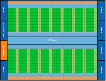
Figure 1.1: Nvidia Fermi Architecture (Source:NVIDIA)
A host interface connects the GPU to the CPU via the PCI-Express bus. The GPU has six 64-bit memory partitions for a 384-bit memory interface supporting up to a total of 6 GB of GDDR4 DRAM memory. The GPU memory hierarchy contains the following levels, from fastest to slowest (see Figure 1.2):
• Register File: In contrast to CPUs, GPUs maintain a much larger register file size of 32K-word per SM. Registers are dedicated to threads once they are assigned to them. This allows multi-thread context switches at clock cycle rate (in a single cycle).
• Configurable On-chip Shared Memory: In the Fermi architecture, each SM has 64 KB of on-chip memory that can be configured as 48 KB of Shared memory with 16 KB of L1 cache or as 16 KB of Shared memory with 48 KB of L1 cache. Shared memory can be treated as a scratch pad that gives programmers more control of data locality.
(Device) Grid
Constant Memory Texture Memory Global Memory
Block (0, 0)
Shared Memory
Local Memory Thread (0, 0) Registers
Local Memory Thread (1, 0) Registers
Block (1, 0)
Shared Memory
Local Memory Thread (0, 0) Registers
Local Memory Thread (1, 0) Registers
Host
Figure 1.2: CUDA Memory Overview (Source:NVIDIA)
• Off-chip memory: This includes global memory, constant memory and texture memory. Constant memory and texture memory use a different cache than the L2 cache. It is sometimes beneficial to map data into constant or texture memory to avoid polluting the L2 cache.
All levels of memory are protected by ECC (error correcting code) in Tesla GPU cards. ECC can correct single bit errors and detect double bit errors.
On the software side, a CUDA program calls parallel kernels. A kernel executes in parallel across a set of parallel threads, which are mapped to different hierarchies, from top to bottom (see Figure 1.3):
• Grid: The GPU instantiates a kernel program on a grid of parallel thread blocks. One kernel maps to one grid of threads. It is at this top level that CUDA threads are created and destroyed. An implicit barrier exists between kernel calls.
• Block: A grid is organized as a set of 1D, 2D or 3D of blocks. A block has a unique ID. Threads inside one block can synchronize and share data through the usage of Shared memory.
Figure 1.3: CUDA Thread Hierarchy (Source:NVIDIA)
branches needs to be executed if threads in the warp deviate. Currently, the size of a warp is 32 threads.
• Thread: Each thread within a thread block executes an instance of the kernel and has a thread ID within its thread block, program counter, registers, per-thread private memory, inputs, and output results.
1.3
Hypothesis
Recent microprocessor architectures are providing rapidly increasing amount of built-in parallelisms. Our research focuses on heterogeneous GPGPUs, which are becoming widely adopted in parallel pro-cessing. This new trend provides new opportunities to rethink the tool chain of programming including languages, programming models and compilation frameworks.
The hypothesis of this dissertation is:
Data parallelism provides the means to exploit the massive throughput of the increasing number
of computation cores featured by today’s microprocessors. A fundamental redesign of the tool chain including languages, programming models and compilation frameworks for data parallelism has the
potential to significantly increase programmability and performance in such environments.
1.4
Organization
The remainder of this document is split into the following parts.
• We assess the benefits of exploiting the computational power of GPUs to study two fundamental problems in document mining, namely to calculate TF-IDF (Term Frequency-Inverse Document Frequency) and cluster a large set of document (Chapter 2). We transform traditional algorithms into accelerated parallel counterparts that can be efficiently executed on many-core GPU archi-tectures. We evaluate our implementations on various platforms ranging from stand-alone GPU desktops to Beowulf-like clusters equipped with contemporary GPU cards. We observe at least one order of magnitude speedups over CPU-only desktops and clusters. This demonstrates the po-tential of exploiting GPU clusters to efficiently solve massive document mining problems. Such speedups combined with the scalability potential and accelerator-based parallelization are unique in the domain of document-based data mining, to the best of our knowledge.
• We propose GStream, a general-purpose, scalable data streaming framework on GPUs, to demon-strate the GPU’s ability to operate on general streaming applications (Chapter 3). We pro-vide powerful, yet concise language abstractions suitable to describe conventional algorithms as streaming problems. We then project these abstractions onto GPUs to fully exploit their in-herent massive data-parallelism. By providing a transparent memory transfer interface, we show that the proposed framework provides flexibility, programmability and performance gains for var-ious benchmarks from a collection of domains, including but not limited to data streaming, data parallel problems and numerical codes.
space. Our proposed framework takes a most concise specification of stencil behavior from the user as a single formula, auto-generates tunable code from it, systematically searches for the best configuration and generates the code with optimal parameter configurations for different GPUs. This auto-tuning approach guarantees adaptive performance for different generations of GPUs while greatly enhancing programmer productivity. Experimental results show that the delivered floating-point performance is very close to previous handcrafted work and outperforms other auto-tuned stencil codes by a large margin.
• In order to automatically exploit data parallelism for current GPUs, we develop a source-to-source compiler framework to convert NESL, a nested data-parallel language, into CUDA code (Chapter 5). As data-parallelism is the fundamental element in NESL, we show how natural it is to fit such languages into SIMT (single instruction multiple threads) environments. Preliminary results indicate that the resulting code still preserves performance advantages over manually written code running on the latest multi-core CPUs.
Chapter 2
Document Clustering on GPU Clusters
2.1
Introduction
Document clustering, or text clustering, is a sub-field of data clustering where a collection of docu-ments are categorized into different subsets with respect to document similarity. Such clustering occurs without supervised information,i.e., no prior knowledge of the number of resulting subsets or the size of each subset is required. Clustering analysis in general is motivated by the explosion of information accumulated in today’s Internet,i.e., accurate and efficient analysis of millions of documents is required within a reasonable amount of time. This trend has resulted in a myriad of clustering algorithms de-veloped lately. A recent flocking-based algorithm [41] implements the clustering process through the simulation of mixed-species birds in nature. In this algorithm, each document is represented as a point in a two-dimensional Cartesian space. Initially set at a random coordinate, each point interacts with its neighbors according to a clustering criterion,i.e., typically the similarity metric between documents. This algorithm is particularly suitable for dynamical streaming data and is able to achieve global optima, much in contrast to our algorithmic solutions [108].
In this chapter, we first solve one of the fundamental problems in document mining, namely that of calculating TF-IDF vectors of documents. The TF-IDF vector is subsequently utilized to quantify docu-ment similarity in docudocu-ment clustering algorithms. We show how to re-design the traditional algorithm into a CPU-GPU co-processing framework and we demonstrate up to 10X speedup over a single-node CPU desktop.
host main memory. Instead, such memory transfers have to be invoked explicitly. The overhead of these memory transfers, even when supported by DMA, can nullify the performance benefits of execution on accelerators. Hence, a thorough design to assure well-balanced computation on accelerators and com-munication / memory transfer to and from the host computer is required,i.e., overlap of data movement and computation is imperative for effective accelerator utilization. Moreover, the inherently quadratic computational complexity in the number of documents and the large memory footprints, however, make efficient implementation of flocking for document clustering a challenging task. Yet, the parallel na-ture of such a model bears the promise to exploit advances in data-parallel accelerators for distributed simulation of flocking.
As a result, we investigate the potential to purse our goal on a cluster of computers equipped with NVIDIA CUDA-enabled GPUs. We are able to cluster one million documents over sixteen NVIDIA GeForce GTX 280 cards with 1GB on-board memory each. Our implementation demonstrates its capa-bility for weak scaling,i.e., execution time remains constant as the amount of documents is increased at the same rate as GPUs are added to the processing cluster. We have also developed a functionally equivalent multi-threaded MPI application in C++ for performance comparison. The GPU cluster im-plementation shows dramatic speedups over the C++ imim-plementation, ranging from 30X to more than 50X speedups.
The contributions of this work are the following:
• We design highly parallelized methods to build hash tables on GPU as a premise to calculate TF-IDF vectors for a given set of documents.
• We apply multiple-species flocking (MSF) simulation in the context of large-scale document clus-tering onGPU clusters. We show that the high I/O and computational throughput in such a cluster meets the demanding computational and I/O requirements.
• In contrast to previous work that targeted GPU clusters [48, 38], our work is one of the first to utilize CUDA-enabled GPU clusters to acceleratemassive data mining applications, to the best of our knowledge.
• The solid speedups observed in our experiments are reportedover the entire application(and not just by comparing kernels without considering data transfer overhead to/from accelerator). They clearly demonstrate the potential for this application domain to benefit from acceleration by GPU clusters.
2.2
Background Description
In this section, we describe the algorithmic steps of TF-IDF and document clustering, and discuss details of the target programming environments.
2.2.1 TF-IDF
Term frequency (TF) is a measure of how important a term is to a document. The ith term’s tf in documentjis defined as:
tfi,j =
ni,j
P
knk,j
(2.1)
whereni,j is the number of occurrences of the term in documentdj and the denominator is the number
of occurrences of all terms in documentdj.
The inverse document frequency (IDF) measures the general importance of the term in a corpus of documents. This is done by dividing the number of all documents by the number of documents containing the term and then taking the logarithm.
idfi =log
|D| |{dj :ti∈dj}|
(2.2)
where |D| is the total number of documents in the corpus and |{dj : ti ∈ dj}| is the number of
documents containing termti.
Then, the TF-IDF value of theith term in documentjis:
tf idfi,j =tfi,j∗idfi (2.3)
The idea of TF-IDF can be extended to compare the similarities of two documentsdi anddj. One
of the simple way is to apply the similarity metric between any pair of documentsiandj:
Simi,j =
X
k
|tf idfk,i−tf idfk,j|2 (2.4)
forkover all terms of both documentiandj. Obviously, the smaller the value is, the more similar these two documents are considered.
local commercial aviation history
unpreced move local commerci aviat histori In an unprecedented move in local commercial aviation history, ...
Build token frequence hash table per document
Remove stopwords & tokenize
Stem word
Calculate Tf−idf
...
...
...
...
...
...
...
...
Build global occurence hash table 1
2
3
4
5
unprecedented move
Figure 2.1: TF-IDF Workflow
cognate words are transformed into one form by applying certain stemming patterns for each. This is necessary to obtain results with higher precision [73]. In step three, the document hash table is built for each document. The<key, value>pairs in the token hash table are the unique words that appear in the document and their occurrence frequencies, respectively. In step four, all of these token hash tables are reduced into one global occurrence table in which the keys remain the same, but values represent the number of documents that contain the associated key. The TF-IDF for each term can be easily calculated by looking up the corresponding values in the hash tables according to Equation 2.3 as seen in step five.
2.2.2 Flocking-based Document Clustering
flocking-based clustering, the behavior of a boid (individual) is flocking-based only on its neighbor flock mates within a certain range. Reynolds [101] describes this behavior in a set of three rules. Letp~jandv~jbe the position
and velocity of boidj. Given a boid noted asx, suppose we have determinedN of its neighbors within radiusr. The description and calculation of the force by each rule is summarized as follows:
• Separation: steer to avoid crowding local flock mates
~
fsep =−
N
X
i ~ px−p~i
r2 i,x
(2.5)
whereri,xis the distance between two boidsiandx.
• Alignment: steer towards the average heading of local flock mates
~
fali=
PN i v~i
N −v~x (2.6)
• Cohesion: steer to move toward the average position of local flock mates
~
fcoh=
PN i p~i
N −p~x (2.7)
The three forces are combined to change the current velocity of the boid. In case of document clustering, we map each document as a boid that participates in flocking formation. For similar neighbor documents, all three forces are combined. For non-similar neighbor documents, only theseparation force is applied.
2.3
Design and Implementation of TF-IDF Calculation
One of the key challenges in algorithmic design for GPGPUs is to keep all processing elements busy. NVIDIA’s philosophy to ensure high utilization is to oversubscribe,i.e., more parallel work is dispatched than there are physical stream processors available. Using latency-hiding techniques, a processor stalled on a memory reference can thus simply switch context to another dispatched work unit.
File Stream
Buffer B File StreamBuffer A
Doc Hash Table Buffer
BuildDocHash_kernel
AddToOccTable_kernel
Global Occ Table Launch
Kernels Disk Read
Sync DMA File Stream
Launch Kernels
Next Batch Disk Read
Sync DMA File Stream Table DMA
Wait Hash
Tokenize_kernel
Async Hash Table DMA Table Pool
Host Hash
barrier barrier
CPU GPU
RemoveAffix_kernel
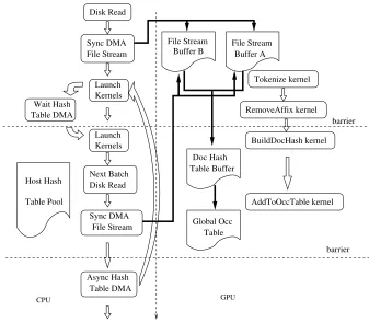
Figure 2.2: CPU/GPU Collaboration Framework
memory at the beginning of each batch process. To reduce the overhead of memory movement, we developed the CPU/GPU collaboration framework shown in Figure 2.2.
In each batch iteration, the CPU thread first launches the two preprocessing kernels (Tokenize kernel and RemoveAffix kernel) asynchronously. Before invoking the next kernels (BuildDocHash kernel and AddToOccTable kernel) that write to the document and global occurrence hash table buffers in the GPU’s global memory, it waits for the completion signal of the previous issued DMA. This DMA saves the document hash tables in the previous batch to host memory. When the GPU is busy generating the document hash tables and inserting tokens into the global occurrence table, the CPU can prefetch the next batch of files from disk and copy them to an alternate file stream buffer. At the end of the batch iteration, the CPU again asynchronously issues a memory copy of the document hash table to the host’s memory. Only in the next batch’s iteration will the completion of this DMA be synchronized. In this manner, part of the DMA time is overlapped with the GPU calculation by (a) double buffering the document raw data in GPU and (b) overlapping the hash table memory copy in the current batch with the stream preprocessing (tokenize and stem kernels) of the next batch [36].
total size key, identity index next key, identity index next key, identity index next key, identity index next key, identity index next key, identity actual token key, identity actual token key, identity actual token key, identity actual token key, identity actual token bucket 0 size
bucket 1 size
bucket N size
bucket 0 first
bucket 1 first
bucket M first
Global Occurence Table Document Hash Table
key, identity actual token bucket usage bucket usage bucket usage
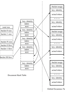
Figure 2.3: Hash Table Data Structures
table differs from the global occurrence table, which resides in GPU global memory but need not be copied to host until the end of execution. Therefore, the data structures of these tables differ slightly as shown in Figure 2.3. Since no hash insertion or deletion operations will be performed afterwards, we store this table as a linked list. The data structure contains a header and an array of entries, which are stored continuously if they belong to the same bucket. The header is used to determine the bucket size and to find the first entry in each bucket. In contrast, the global hash table consists of a big array of entries evenly divided into buckets. Because the number of unique terms is considered limited no matter how large the corpus size is, the number of buckets and the bucket size can be chosen sufficiently large to avoid possible bucket overflows.
global occurrence table where the actual term is saved. To reduce the number of hash key computations at hash insertion and during hash searches, the key is saved as an “unsigned long” in both hash tables. To further reduce the probability of hash collisions (two terms sharing the same key), another field called identity is added as an “unsigned int” to help differentiate terms. The identity is then constructed as
(term length <<16)|(f irst char <<8)|(last char).
Upon investigation, we determined that atomic operations supported by certain GPUs via CUDA are facilitating the construction of a concise document hash table without adversely affecting the parallelism of the algorithm. We alternatively provide another method to generate the same hash table for GPUs without support for atomic operations. Even though the latter method is slower than the first, it is required for GPU devices that do not have atomic operation support (i.e., devices with CUDA compute capability 1.0 or earlier).
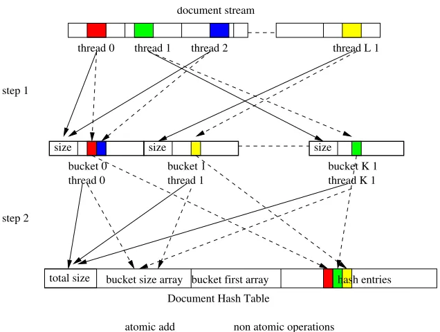
2.3.1 Hash Table Updates using Atomic Operations
Access to hash table entries viaatomic operations is realized in two steps as depicted in Figure 2.4. In the first step, the document stream is evenly distributed to a set of CUDA threads. The number of threads,L, is chosen explicitly to maximize GPU’s utilization. A buffer storing the intermediate hash table, which is close to the structural layout of the global occurrence table, but with a smaller number of bucketsK, is used to sort terms by their bucket IDs. Every time a thread encounters a new term in the stream and obtains its bucket ID, it issues an atomic increment (atomic-add-one) operation to affect the bucket size. (Notice that the objective of this algorithmic TF-IDF variant is not to identify identical terms. Instead, its chief objective is to compute a similarity metric.) If we assume that terms are distributed randomly, then contention during the atomic increment operation is the exception,i.e., threads of the same warp are likely atomically incrementing disjoint bucket size entries.
In the next step, the intermediate hash table is reduced to the final, more concise document hash table shown in Figure 2.3. Each CUDA thread traverses one bucket in the intermediate hash table, detects duplicate terms, and, if finds a new term, reserves a place in the entry array by atomically incrementing the total size. It then pushes the new entry into the header of the linked bucket list. Since different threads operate on disjoint buckets, each linked list per bucket is accessed in mutual exclusion, which guarantees absence of write conflicts between threads.
2.3.2 Hash Table Updates without Atomic Operations
step 2
thread 0 thread 1 thread 2 thread L−1
total size
atomic add non−atomic operations
bucket size array bucket first array hash entries
Document Hash Table bucket 0 bucket 1
size size size
thread 1 thread 0
bucket K−1 thread K−1 document stream
step 1
Figure 2.4: Building a Hash Table with Atomic Operations
Because terms have been grouped by their keys in step 1, there will be no write conflicts between threads at this step either. The bucket size information is processed in step 3 to finally merge sub-tables to compose the final document hash table.
2.3.3 Discussions
The two procedures detailed above to handle hash tokens in a document do not require information from any other documents. Thus, each document can be processed simultaneously and independently in different GPU blocks. With a sufficiently large number of documents, we can fully utilize the GPU cores and exploit NVIDIA’s latency hiding on memory references through oversubscription. However, in the first step of the second method, the number of packets M per document is delimited due to memory constraint and the efficiency of the following steps. We choose a value of M = 16 in our implementation. To compensate for this constraint, we can spawn more threadsLin the first method, e.g., by choosingL= 512. This constraint on parallelism results in a non-atomic approach that is slower than its atomic variant.
0000 0000 1111 1111 0000 0000 0000 1111 1111 1111 0000 0000 0000 1111 1111 1111 000 000 111 111 000 000 111
111
000
111
000 000 111 111 000 000 000 111 111 111 000 000 000 111 111 111 000 000 111 111 000 000 000 111 111 111 000 000 000 111 111 111
000
000
111
111
000
000
111
111
000
111
bucket 0 totalbucket 0, 1 total bucket 0..K−1 total bucket 0 total bucket 1 total bucket K−1 total total size 00 00 00 00 11 11 11 11 0 0 0 0 1 1 1 1 00 00 00 00 11 11 11 11 0 0 0 0 1 1 1 1 00 00 00 00 11 11 11 11 0 0 0 0 1 1 1 1 0 0 0 0 1 1 1 1 00 00 00 00 11 11 11 11 0 0 0 0 1 1 1 1 00 00 00 00 11 11 11 11
0
0
0
1
1
1
00
00
00
11
11
11
0
0
0
1
1
1
0000 0000 0000 1111 1111 1111 0000 0000 0000 1111 1111 11110000
0000
1111
1111
thread 0 thread 1 thread 2 document stream
thread 0 thread 1 sub hash tables
step 1
bucket 0 bucket 1
step 2 prefix sum 0 thread K−1 bucket K−1 thread M−1 step 3
bucket size array bucket first array Document Hash Table
0000 0000
1111 1111
hash entries
Figure 2.5: Building a Hash Table without Atomic Operation
not exceed more than 10K words, documents fits in memory for our implementation. This framework is even suitable for arbitrarily large corpus sizes as we could reused without changes both intermediate hash tables and the document hash table, the latter of which is flushed to host memory for each batch of files.
2.4
Design and Implementation of Document Clustering
2.4.1 Programming Model for Data-parallel Clusters
We have developed a programming model targeted at message passing for CUDA-enabled nodes. The environment is motivated by two problems that surface when explicitly programming with MPI and CUDA abstraction in combination:
• Sharing one GPU card among multiple CPU threads can improve the GPU utilization rate. How-ever, explicit multi-threaded programming not only complicates the code, but may also result in inflexible designs, increased complexity and potentially more programming pitfalls in terms of correctness and efficiency.
To address these problems, we have devised a programming model that abstracts from CPU/GPU co-processing and mitigates the burden of the programmer to explicitly program data movement across nodes, host memories and device memories. We next provide a brief summary of the key contributions of our programming model (see [124] for a more detailed assessment):
• We have designed adistributed object interfaceto unify CUDA memory management and explicit message passing routines. The interface enforces programmers to view the application from a data-centric perspective instead of a task-centric view. To fully exploit the performance potential of GPUs, the underlying run-time system can detect data sharing within the same GPU. Therefore, the network pressure can be reduced.
• Our model provides the means to spawn a flexible number of host threads for parallelization that mayexceedthe number of GPUs in the system. Multiple host threads can be automatically assigned to the same MPI process. They subsequently share one GPU device, which may result in higher utilization rate than single-threaded host control of a GPU. In applications where CPUs and GPUs co-process a task and a CPU cannot continuously feed enough work to a GPU, this sharing mechanism utilizes GPU resources more efficiently.
• An interface for advanced users to control thread scheduling in clusters is provided. This interface is motivated by the fact that the mapping of multiple threads to physical nodes affects performance depending on the application’s communication patterns. Predefined communication patterns can simply be selected so that communication endpoints are automatically generated. More complex patterns can be supported through reusable plug-ins as an extensible means for communication.
We have designed and implemented the flocking-based document clustering algorithm in GPU clus-ters based on this GPU cluster programming model. In the following, we discuss several application-specific issues that arise in our design and implementation.
2.4.2 Preprocessing
The prerequisite of document clustering is to have a standard means to measure similarities between any two documents. While the TF-IDF concept exactly matches this need, there are two practical issues when targeting clusters:
• The TF-IDF calculation cannot start until all documents have been processed and inserted in the global occurrence table. Therefore, it is not suited for stream processing.
A new term weighting scheme called term frequency-inverse corpus frequency (TF-ICF) has been proposed to solve the above problems at the scale of massive amounts of documents [100]. It does not require term frequency information from other documents within the processed document collections. Instead, it pre-builds the ICF table by sampling a large amount of existing literature off-line. Selection of corpus documents for this training set is critical as similarities between documents of a later test set are only reliable if both training and test sets share a common base dictionary of terms (words) with a similar frequency distribution of terms over documents. Once the ICF table is constructed, ICF values can be looked up very efficiently for each term in documents while TF-IDF would require dynamic calculation of these values. The TF-ICF approach enables us thus to generate document vectors in linear time.
2.4.3 Flocking Space Partition
The core of the flocking simulation is the task of neighborhood detection. A sequential implementation of the detection algorithm has O(N2) complexity due to pair-wise checking of N documents. This
simplistic design can be improved through space filtering, which prunes the search space for pairs of points whose distances exceed a threshold.
One way to split the work into different computational resource is to assign a fixed number of documents to each available node. Suppose there areN documents andP nodes. In every iteration of the neighborhood detection algorithm, the positions of local documents are broadcast to all other nodes. Such partitioning results in a lower communication overhead proportional to the number of nodes, and the detection complexity is reduced linearly byP per node for a resulting overhead ofO(N2/P).
Sliced space partitioning not only splits the work nearly evenly among computing nodes but also reduces the algorithmic complexity in sequential programs. Neighborhood checks across different nodes are only required for neighbor documents within the boundaries, not for internal documents. Therefore, on average, the detection complexity on each node reduces toO(N2/P2)for slides partitioning, which is superior to traditional partitioning withO(N2/P).
GPU0
GPU1
GPUn−1 r r r
r
r
r
...
Migrating Doc
Internal Doc
Neighbor Doc
Figure 2.6: Simulation Space Partition
2.4.4 Document Vectors
An additional benefit of MSF simulation is the similarity calculation between two neighbor documents. Similarities could be pre-calculated between all pairs and stored in a triangular matrix. However, this is infeasible for very largeN because of a space complexity of O(N2/2), which dauntingly exceeds the address space of any node asN approaches a million. Furthermore, devising an efficient partition scheme to store the matrix among nodes is difficult due to the randomness of similarity look-ups between any pair of nearby documents. Therefore, we devote one kernel function to calculating similarities in each iteration. This results in some duplicated computations, but this method tends to minimize the memory pressure per node.
The data required to calculate similarities is a document vector consisting of an index of each unique word in the TF-ICF table and its associated TF-ICF values. To compute the similarity between two documents, as shown in Equation (2.4), we need a fast method to determine if a document contains a word given the word’s TF-ICF index. Moreover, the fact that we need to move the document vector between neighbor nodes also requires that the size of the vector should be kept small.
word in the TF-ICF table. This data structure combines the minimal memory usage with a fast parallel searching algorithm. Riech [103] describes an efficient algorithm to calculate the Euclidean similarities between any two sorted arrays. But this algorithm is iterative in nature and not suitable for parallel processing.
We develop an efficient CUDA kernel to calculate the similarity of two documents given their sorted document vectors as shown in Algorithm 1. The parallel granularity is set so that each block takes one pair of documents. Document vectors are split evenly by threads in the block. For each assigned TF-ICF value, each thread determines if the other document vector contains the entry with the same index. Since the vectors are sorted, a binary search is conducted to lower the algorithmic complexity logarithmic time. A reduction is performed at the end to accumulate differences.
2.4.5 Message Data Structure
In sliced space partitioning, each slice is responsible to generate two sets of messages for the slices above and below. The corresponding message data structures are illustrated in Figure 2.7. The doc-ument array contains a header that enumerates the number of neighbors and migrating docdoc-uments in the current slice. Their global indexes, positions and velocities are stored in the following array for neighborhood detection in a different slice. Due to the various sizes of each document’s TF-ICF vector and the necessity to minimize the message size, we concatenate all vectors in a vector array without any padding. The offset of each vector array is stored in a metadata offset array for fast access. This design offers efficient parallel access to each document’s information.
2.4.6 Optimizations
The algorithmic complexity of sliced partitioning decreases quadratically with the number of partitions (see Section 2.4.3). For a system with a fixed number of nodes, a reduction in complexity could be achieved by exploiting multi-threading within each node. However, in practice, overhead increases as the number of partitions become larger. This is particularly this case for communication overhead. As we will see in Section 2.5, the effectiveness of such performance improvements differs from one system to another.
Algo 1: Document Vector Similarity (CUDA Kernel) // calculate the similarities between two DocVecs
device voiddocVecSimilarity(DocVec∗lhs, DocVec∗rhs,float∗output){ floatsim(0.0f);
floatcommonSim(0.0f);
for(inti = 0; i<lhs→NumEntries; i += blockIdx.x){ floattficf = biSearch(entry, rhs→vectors);
sum += pow(entry→tficf−tficf, 2); commonSim += pow(tficf, 2);
}
// ... reduce to threadIdx.x(0), store in sum syncthreads();
if(threadIdx.x == 0){
sum−= commonSim; sum = sqrtf(sum); // write to global memory
∗output = sum;
} }
device floatbiSearch(VecEntry∗entry, DocVector∗vector){ intidx = entry→index;
intleftIndex = 0;
intrightIndex = vector→NumEntries; intmidIndex = vector→NumEntries/2; while(true){
intdocIdx;
docIdx = vector→vectors[midIndex].index; if(docIdx<idx)
leftIndex = midIndex + 1; else if(docIdx>idx)
rightIndex = midIndex−1; else
break;
if(leftIndex>rightIndex) return0.0f;
midIndex = (leftIndex + rightIndex)/2;
}
returnvector→vectors[midIndex].tficf;
...
vector offset Neighbor1 vector offset
Migrating0 vector offset Migrating1 vector offset
...
...
Neighbor0 doc vector
Neighbor1 doc vector Array
Vector Offset
Neighbor0 (idx, pos, vel)
Migrating0 doc vector
Migrating1 doc vector Neighbor0
(idx, pos, vel)
...
...
Document Array
Vector Array
NumNeighbors
(idx, pos, vel) Neighbor1
...
NumNeighbors NumMigratings
NumMigratings
Neighbor0
Figure 2.7: Message Data Structures
migrated documents, we expect the execution time for sub-function (a) to be much larger than that of (b) or (c). From the system’s point of view, either the communication or neighbor detection functions affects the overall performance.
One of the problems in simulating massive documents via the flocking-based algorithm is that as the virtual space size increases, the probability of flock formation diminishes as similar groups are less likely to meet each. In nature-inspired flocking, no explicit effort is made within simulations to combine similar species into a unique group. However, in document clustering, we need to make sure each cluster has formed onlyone groupin the virtual space in the end without flock intersection. We found that an increase in the number of iterations helps in achieving this objective. We also dynamically reduce the size of the virtual space throughout the simulation. This increases the likelihood of similar groups to merge when they become neighbors.
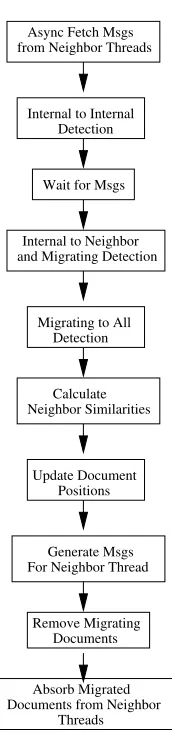
2.4.7 Work Flow
Internal-to-internal document detection can be performed in parallel with message passing (see Sec-tion 2.4.6). The other two detecSec-tion routines, in contrast, are serialized with respect to message ex-changes. Once all neighborhoods are detected, we calculate the similarities between the documents belonging to the current thread and their detected neighbors. These similarity metrics are utilized to update the document positions in the next step where the flocking rules are applied.
Async Fetch Msgs
Internal to Internal Detection
Wait for Msgs
Internal to Neighbor and Migrating Detection
Migrating to All Detection
Update Document Positions Neighbor Similarities
Calculate
Generate Msgs For Neighbor Thread
Remove Migrating Documents
Absorb Migrated Documents from Neighbor
Threads from Neighbor Threads
Figure 2.8: Work Flow for a Thread in Each Iteration
performed in the last three steps in Figure 2.8.
Table 2.1: Experiment Platforms
16 GPUs (NCSU) 16 CPUs (NCSU) 3 GPUs (ORNL) 3 CPUs (ORNL)
Nodes 16 16 4 4
CPU Cores AMD Athlon Dual AMD Athlon Dual Intel Quad Q6700 Intel Quad Q6700
CPU Frequency 2.0 GHz 2.0 GHz 2.67 GHz 2.67 GHz
System Memory 1 GB 1 GB 4 GB 4 GB
GPU 16 GTX 280s Disabled 3 Tesla C1060 Disabled
GPU Memory 1 GB N/A 4 GB N/A
Network 1 Gbps 1 Gbps 1 Gbps 1 Gbps
2.5
Experimental Results
2.5.1 Experiment Setups
We conduct two independent sets of experiments to show the performance of our TF-IDF and document clustering results.
TF-IDF experiments are conducted on a stand-alone desktop in two configurations: with GPU en-abled and disen-abled. When the GPU is disen-abled, we assess the performance of a functionally equivalent CPU baseline version (single-threaded in C/C++). The test platform utilizes Fedora 8 Core Linux with a dual-core AMD Athlon 2 GHz CPU with 2 GB of memory. The installation includes the CUDA 2.0 beta release and NVIDIA’s Geforce GTX 280 as GPU devices. The test input data is selected from Internet news documents with variable sizes ranging from around 50 to 1000 English words (after stop-word removal). The average number of unique word in each article is about 400 words.
2.5.2 TF-IDF Experiments
In TF-IDF experiments, we first compare the execution time for one batch of 96 files. The individual module speedup and their percentages in total are shown in Figure 2.9 and Figure 2.10.
Notice that the speedup on the y-axis of Figure 2.9 is depicted on a logarithmic scale. Compared to the CPU baseline implementation, we achieve more significant speedups for those modules engaged in the preprocessing phase (factor of 30 times faster in tokenize and 20 times faster in strip affixes kernels) than for those at the hash table construction phase (around 3 times faster in both document hash table and occurrence table insertion kernels). The limits in speedup during the latter are due to the multi-step hash table construction algorithms described in Section 2.3. The algorithm has certain overheads that the CPU benchmark does not contain. These overheads include (a) the construction of intermediate or hash sub-tables; (b) branching penalties suffered from the SIMD nature of GPU cores due to the imbalance in the distribution of tokens for a hash table’s buckets; and (c) non-coalesced global memory access patterns as a result of the randomness of the hash key generation. Furthermore, the kernel for occurrence table insertion does not fully exploit all GPU cores because insertion is inherently serialized over files to avoid write conflicts within the same hash table bucket.
0.1 1 10 100 1000 10000 100000
Disk I/O Stopword Stem Doc HashOcc Table Tfidf DMA
Module Execution Time (us)
Module CPU/GPU Execution Time CPU
GPU
0.1 1 10 100
Disk I/O Stopword Stem Doc HashOcc Table Tfidf DMA
Speedups
Module GPU Speedup
We also observe a reduction in the calculation time to the extent that the DMA overhead has become the largest contributor to overall time in asingle batchscenario accounting for almost half of the total execution time. The combined time with disk I/O exceeds the total kernel execution time on GPU.
CPU GPU GPU/CPU
% of total
Tokenize Strip Affixes Doc Hash Occ Table Tfidf Disk I/O Stream Dma Hash Gather Dma Hash tfidf Dma memcpy
Figure 2.10: Per-Module Contribution to Overall Execution Time
The observation above gives us the motivation to mitigate the memory overhead by double buffering the stream and hash tables when the corpus size gets larger. While we cannot hide the DMA overhead of a first batch, the DMA time of subsequent batches can be completely overlapped with the computa-tional kernels in amulti-batchscenario. Figure 2.11 shows the execution time of CPU and CUDA with different corpus sizes.
The execution time of the two methods (both with and with the use of atomic instructions) are measured. With almost perfect parallelization between GPU calculation and data migration, we can hide almost all the kernel execution time in the DMA transfer and disk I/O time, which indicates a lower bound of the execution time. As a result the the asymptotic average batch processing time is almost half comparing to the single batch execution time, in which case the calculation and DMA cannot be overlapped. We also observe that the overall acceleration rates are 9.15 and 7.20 times faster than the CPU baseline.
2.5.3 Flocking Behavior Visualization
0.1 1 10 100 1000 10000 100000
100 1000 10000 100000
Execution Time (ms)
Corpus Size
Execution Time with Different Corpus Size(ms)
CPU GPU(with atomic instruction) GPU(without atomic instruction)
Figure 2.11: Execution Time with Different Corpus Size
four GPUs. Initially, documents are assigned at random coordinates in the virtual plane. After only 50 iterations, we observe an initial aggregation tendency. We also observe that the number of non-attached documents tends to decrease as the number of iterations increases. In our experiments, we observe that 500 iterations suffice to reach a stable state even for as many as a million documents. Therefore, we use 500 iterations throughout the rest of our experiments.
(a) Initial State (b) At Iteration 50 (c) At Iteration 500
Figure 2.12: Clustering 20K Documents in 4 GPUs
factor of the similarity threshold used throughout the simulation. The smaller the threshold is / the more strict the similarity check is, the more groups we will be formed through flocking.
2.5.4 Document Clustering Performance
We first compare the performance of individual kernels on an NVIDIA GTX 280 GPU hosted on a AMD Athlon 2 GHz Dual Core PC. We focus on two of the most time-consuming kernels: detecting neighbor documents (detection for short) and neighbor document similarity calculation (similarity for short). Only the GPU kernel is measured in this step. The execution time is averaged over 10 independent runs. Each run measures the first clustering step (first iteration in terms of Figure 2.12) to determine the speedup over the CPU version starting from the initial state. The speedup at different document sizes is shown in Figure 2.13. We can see that the similarity kernel on the GPU is about 45 times faster than on a CPU at almost all document sizes. For the detection kernel, the GPU is fully utilized once the document size exceeds 20,000, which gives a raw speedup of over 300X.
0 50 100 150 200 250 300 350
0 10000 20000 30000 40000 50000 60000
GPU/CPU Kernel Speedup
Number of Documents
Similarity Kernel Detection Kernel
Figure 2.13: Speedups for Similarity and Detection Kernels
We next conducted experiments on two clusters located at NCSU and ORNL. On both clusters, we conducted test with and without GPUs enabled (see hardware configurations in Table 2.1). The NCSU cluster consists of sixteen nodes with CPUs and GPUs of lower RAM capacity for both CPU and GPU, while the ORNL cluster consists of fewer nodes with larger RAM capacity. As mentioned in Section 2.4.1, our programming model supports a flexible number of CPU threads that may exceed the number of GPUs on our platform. Thus, multiple CPU threads may share one GPU. In our experiments, we assessed the performance for both one and two CPU threads per GPU.
over the execution for both one and two CPU threads per GPU. The error bar shows the actual execution time: the maximum/minimum represent one/two CPU threads per GPU, respectively. With increasing of number of nodes, execution time decreases and the maximal number of documents that can be processed at a time increases. With 16 GTX 280s, we are able to cluster one million documents within twelve minutes. The relative speedup of the GPU cluster over the CPU cluster ranges from 30X to 50X. As mentioned in Section 2.4.6, changing the number of threads sharing one GPU may cause a number of conflicts in resource. The benefit of multi-threading in this cluster is only moderate with only up to a
10%performance gain.
10 100 1000 10000 100000 1e+06
0 200 400 600 800 1000
Execution Time (sec)
Document Population (X 1K)
4 CPUs 8 CPUs 12 CPUs 16 CPUs 4 GPUs 8 GPUs 12 GPUs 16 GPUs
Figure 2.14: Execution Time on GTX 280 GPUs
Though the ORNL cluster contains fewer nodes, its single-GPU memory size is four times larger than that of the NCSU GPUs. This enables us to cluster one million documents with only three high-end GPUs. The execution time is shown in Figure 2.15. The performance improvement resulting for two CPU threads per GPU is more obvious in this case: at one million documents, three nodes with two CPU threads per GPU run20%faster than the equivalent with just one CPU thread per GPU. This follows the intuition that faster CPUs can feed more work via DMA to GPUs.
10 100 1000 10000 100000 1e+06
0 200 400 600 800 1000
Execution Time (sec)
Document Population (X 1K)
2 CPUs 3 CPUs 2 GPUs 3 GPUs
Figure 2.15: Execution Time on Tesla C1060 GPUs
with a lower gradient before increasing rapidly,e.g., between 200k and 500k documents for 16 nodes (GPUs).
We next study the effect of utilizing point-to-point messages for our simulation algorithm. Because messages are exchanged in parallel with the neighborhood detection kernel for internal documents, the effect of communication is determined by the ratio between message passing time and kernel execution time: If the former is less than the latter, then communication is completely hidden (overlapped) by computation. In an experiment, we set the number of documents to 200k and vary the number of nodes from 4 to 16. We assess the execution time per iteration by averaging the communication time and kernel time among all nodes. The result is shown in Figure 2.17. For the GPU cluster, kernel execution time is always less than the message passing time. For the CPU cluster, the opposite is the case.
Table 2.2: Fraction of Communication in GPU and CPU Clusters (GPU/CPU)[in %]
Docs(k) 5 10 20 50 100 200 500 800 1000
4 nodes 74/9 67/8 64/5 58/3 52/1.5 49/0.9 NA NA NA 8 nodes 67/12 71/11 65/8 68/6 62/3.5 56/2 52/1.2 NA NA 12 nodes 67/17 69/12 68/10 71/8 68/6 63/3 57/1.4 54/1.2 NA 16 nodes 63/18 63/13 71/12 69/9 65/7 66/4.2 59/1.9 60/1.5 55/1.1
Figure 2.16: Speedups on NCSU cluster
with that of CPU cluster’s communication time, even though the latter only covers pure network time as no host/device DMA is required. This implies that internal PCI-E memory bus is not a bottleneck for GPU clusters in our experiments, which is important for performance tuning efforts. The causes for this finding are: (a) Network bandwidth is much lower than PCI-E memory bus bandwidth; and (b) messages are exchanges at roughly the same time on every node at each iteration, which may cause network congestion.
10 100 1000 10000 100000
4 6 8 10 12 14 16
Average Time Per Iteration (ms)
Number of Nodes
Message Passing and DMA on GPU Cluster Detection Kernel on GPU Cluster Message Passing on CPU Cluster Detection Function on CPU Cluster
Figure 2.17: Communication and Computation in Parallel
2.6
Related Work
Our acceleration approach over CUDA to calculate document-level TF-IDF values uncovers yet an-other area of potential for GPUs where they outperform general-purpose CPUs. While it has been demonstrated that CUDA can significantly speedup many computationally intensive applications from domains such as scientific computation, physics and molecular dynamics simulation, imaging and the finance sector [51, 92, 105, 42, 6, 63], acceleration is less commonly used in other domains, especially those with integer-centric workloads, with few exceptions[57, 58]. This is partly due to the perception that fast (vector) floating-point calculation are the major contributor to performance benefits of GPUs. However, careful parallel algorithmic design may results in significant benefits as well. This is the premise of our work for text search workload deployment on GPUs.
Related research to document clustering can be divided into two categories: (1) fast simulation of group behavior and (2) GPU-accelerated implementations of document clustering.
Recently, data-parallel co-processors have been utilized to accelerate many computing problems, including some in the domain of massive data clustering. One successful acceleration platform is that of Graphic Processing Units (GPUs). Paralleldatamining on a GPU was assessed early on by Cheet al. [34], Fanget al. [49] and Wuet al. [119]. These approaches rely on k-means to cluster a large space of data points. Since the size of a single point is small (e.g., a constant-sized vector of floating point numbers to represent criteria such as similarity in our case), memory requirements are linear to the size of individuals (data points), which is constrained by the local memory of a single GPU in prac-tice. Previous research has demonstrated more than five times speedups using a single GPU card over a single-node desktop for several thousands documents [32]. This testifies to the benefits of GPU archi-tectures for highly parallel, distributed simulation of individual behavioral models. Nonetheless, such accelerator-based parallelization is constrained by the size of the physical memory of the accelerating hardware platform,e.g., the GPU card.
2.7
Conclusion
In this chapter, we present a complete application-level study of using GPUs to accelerate data-intensive document clustering algorithms.
We first propose a hardware-accelerated variant of the TF-IDF rank search algorithm exploiting GPU devices through NVIDIA’s CUDA. We then develop two highly parallelized methods to build hash tables, one with and one without support of atomic instructions. Even though floating-point calculations are not dominating this text mining domain and its text processing characteristics limit the effectiveness of GPUs due to non-synchronized branching and diverging, data-dependent loop bounds, we achieve a significant speedup over the baseline algorithm on a general-purpose CPU. More specifically, we achieve up to a 30-fold speedup over CPU-based algorithms for selected phases of the problem solution on GPUs with overall wall-clock speedups ranging from six-fold to eight-fold depending on algorithmic parameters.
Chapter 3
GStream: A General-Purpose Data
Streaming Framework on GPU Clusters
3.1
Introduction
Stream processing has established itself as an important application area that is driving the consumer side of computing today. While traditionally used in video encoding/decoding scenarios, other applica-tion areas, such as data analysis and computaapplica-tionally intensive tasks are also discovering the benefits of the streaming paradigm. High computational demands by streaming have been met by general-purpose architectures via multicores. But with no end in sight for these inflating demands, conventional architec-tures are struggling to keep up. We already see significant increases in power and resource management costs particularly for homogeneous general-purpose multicores. Heterogeneous architectures with ac-celerators, such as GPUs, offer a viable alternative to meet the demand in computing as they deliver not only higher cost and power efficiency but also higher performance and scalability.
These performance potentials of GPUs originate from architectural design and programming strate-gies in favor of massive data parallelism. Today’s latest generation of GPUs features hundreds of stream processing units capable of supporting much more data parallelism than a CPU does. The NVIDIA GPU programming model CUDA encourages users to create light-weight software threads at the scale of tens of thousands, which is orders of magnitude larger than the maximal hardware concurrency inside the GPU. This over-subscription of software threads relative to the hardware parallelism allows latency hiding mechanisms to be realized that mitigate the effects of the memory wall [120].