R E S E A R C H
Open Access
Numerical approximation for the solution
of linear sixth order boundary value
problems by cubic B-spline
A. Khalid
1,2, M.N. Naeem
2, P. Agarwal
3,4*, A. Ghaffar
5, Z. Ullah
6and S. Jain
7*Correspondence:
3Department of Mathematics,
Anand International College of Engineering, Jaipur, India
4International Centre for Basic and
Applied Sciences, Jaipur, India Full list of author information is available at the end of the article
Abstract
In the current paper, authors proposed a computational model based on the cubic B-spline method to solve linear 6th order BVPs arising in astrophysics. The prescribed method transforms the boundary problem to a system of linear equations. The algorithm we are going to develop in this paper is not only simply the approximation solution of the 6th order BVPs using cubic B-spline, but it also describes the estimated derivatives of 1st order to 6th order of the analytic solution at the same time. This novel technique has lesser computational cost than numerous other techniques and is second order convergent. To show the efficiency of the proposed method, four numerical examples have been tested. The results are described using error tables and graphs and are compared with the results existing in the literature.
MSC: 34K10; 34K28; 42A10; 65D05; 65D07
Keywords: Linear sixth order BVPs; Numerical approximation; Cubic B-spline; Absolute relative error
1 Introduction
The applications of boundary value problems (BVPs) are almost unlimited, and they play an important role in all the branches of science, engineering, and technology. They are ap-plied to model many systems in several fields of science and engineering. In recent years, there has been significant advancement in solving problems related to a system of linear and nonlinear partial and ordinary differential equations concerning boundary conditions (BC). Two point nonlinear BVPs often cannot be solved by analytical techniques. With cumulative interest in finding solutions to linear/nonlinear BVPs has come an increas-ing requirement for solution techniques. In the present paper, we will study the algebraic results of the following linear 6th order BVP:
w(6)(z) +a
1(z)w(5)(z) +a2(z)w(4)(z) +a3(z)w(3)(z)
+a4(z)w(2)(z) +a5(z)w(1)(z) +a6(z)w(z) =f(z), z∈[a,b] (1)
with boundary conditions
w(m)(a) =αm, w(m)(b) =βm, m= 0, 1, 2, (2)
whereα0,α1,α2andβ0,β1,β2are given real constants, (ai(z);i= 1, 2, . . . , 6), andf is con-tinuous on the given interval [a,b].
A variety of numerical methods [1,2,4,5,8,9,11,12,16,31] have been presented to solve BVPs problem, e.g., global phase-integral methods, shooting methods, sinc-Galerkin methods, splines methods, finite difference methods, finite element methods, variational iteration, the collocation methods, and other numerical techniques.
In [23], a variation of parameter technique was used for solving sixth order boundary value problems. Perturbation method for nonlinear engineering problems was specified in [24]. Homotopy perturbation technique for solving linear and nonlinear sixth order boundary value problems was described in [25]. In [26], algebraic results of 6th order BVPs were originated by applying non-polynomial spline method. Neural networks mimic the learning procedure of the human brain in order to excerpt designs from ancient data as de-fined in [27]. These networks are rehabilitated into 6th order boundary value problems and then resolved by diverse approaches for precise and estimated results. Numerical meth-ods for sixth order boundary value problems were discussed in [32]. In [33], the authors established a family of algebraic procedures for the solutions of 6th order boundary value problems with application to Benard layer eigenvalue problems. Numerical solutions of fifth and sixth order nonlinear boundary value problems by Daftardar–Jafari method were found in [34]. Wazwaz in [35] used decomposition and modified domain decomposition approaches to examine the solution of 6th order boundary value problems.
Discrete methods, e.g., Adomian decomposition, shooting, homotopy-perturbation, fi-nite differences, and variational-iterative technique, only obtained the discrete approxi-mate values of dependent variabley(x). We require further data processing procedures to acquire exact fitted curve to data. For the case of spline approximation or interpolation approaches the dependent variabley(x) is supposed to be piecewise polynomial which in-volves at least piecewise higher order derivatives of the functionf(x,y,y). To overcome these shortcomings, several researchers [3,6,7,10,13–15,17–22,28–30] introduced the spline/subdivision based methods for the solution of BVPs. However, the higher order problems have not been solved by spline/subdivision techniques. This motivates us to solve 6th order boundary value problems by spline. This paper does not only introduce a numerical approximation based on cubic B-spline for the solution of linear 6th order BVPs, but it also describes the estimated derivatives of 1st order to 6th order of the ana-lytic solution at the same time. This novel technique has lesser computational cost than numerous other techniques and is second order convergent.
2 Materials and methods
2.1 Fundamentals of cubic B-splines
The assumed choice of independent variable is [a,b]. For an intervalΩ= [a,b], we divide it intonsubintervalsΩi= [zi,zi+1] (i= 0, 1, . . . ,n– 1) by the equidistant knots, and for this range we select equidistant points assumed by
Ω={a=z0,z1,z2, . . . ,zn=b}, separately sub-interval (zi,zi+1). The basis function is defined as
B–1(z) = 1
Consequently, now for an assumed function w(z) there happened to be a distinctive cubic B-splines(z) =in=–1+1 liBi(z) satisfying the interpolating conditions:
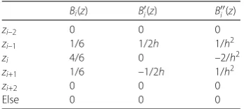
Table 1 Values ofBi(z),Bi(z), andBi(z) at the knots are acquired by the Taylor series expansion
Mi+1–Mi–1
and following the above, we have the Taylor series expansion forw(6)(z) at the selected collocation points with central difference as follows:
Using the above two equations and Eq. (6) in Eq. (9), we have
Using the above equations, we have
1
Neglecting the error order, we have
w(6)(zi) =s(6)(zi) =
li+3– 6li+2+ 15li+1– 20li+ 15li–1– 6li–2+li–3
h6 . (10)
2.2 Cubic B-spline solutions of sixth order BVP
Letw(z) =s(z) =in=–1+1 liBi(z) be the approximate solution of sixth order BVP
w(6)(z) +a1(z)w(5)(z) +a2(z)w(4)(z) +a3(z)w(3)(z)
+a4(z)w(2)(z) +a5(z)w(1)(z) +a6(z)w(z) =f(z), z∈[a,b]
with boundary conditions
whereα0,α1,α2andβ0,β1,β2are given real constants (ai(z);i= 1, 2, . . . , 6) andf is con-tinuous on the given interval [a,b].
w(6)(zi) +a1(zi)w(5)(zi) +a2(zi)w(4)(zi) +a3(zi)w(3)(zi)
+a4(zi)w(2)(zi) +a5(zi)w(1)(zi) +a6(zi)w(zi) =f(zi), z∈[a,b]. (11)
Using Eqs. (8) and (10) in Eq. (11), we have
li+3– 6li+2+ 15li+1– 20li+ 15li–1– 6li–2+li–3
h6
+a1(zi)
li+3– 4li+2+ 5li+1+ 5li–1+ 4li–2–li–3 2h5
+a2(zi)
li+2– 4li+1+ 6li– 4li–1+li–2
h4 +a3(zi)
li+2– 2li+1+ 2li–1–li–2 2h3
+a4(zi)
li+1– 2li+li–1
h2 +a5(zi)
li+1–li–1
2h +a6(zi)
li–1+ 4li+li+1 6
=fi(zi), z∈[a,b].
Simplifying
6(li+3– 6li+2+ 15li+1– 20li+ 15li–1– 6li–2+li–3) + 3ha1(zi)(li+3– 4li+2+ 5li+1
+ 5li–1+ 4li–2–li–3) + 6h2a2(zi)(li+2– 4li+1+ 6li– 4li–1+li–2)
+ 3h3a3(zi)(li+2– 2li+1+ 2li–1–li–2) + 6h4a4(zi)(li+1– 2li+li–1)
+ 3h5a5(zi)(li+1–li–1) +h6a6(zi)(li–1+ 4li+li+1)
= 6h6fi(zi), z∈[a,b]. (12)
By solving Eq. (12) we will have a linear system of (n– 3) linear equations (i= 2, 3, . . . ,n– 2) with (n+ 3) unknownsli, wherei= –1, 0, 1, . . . ,n+ 1, so six more equations are desirable. By the boundary conditions atz=a, we get
w(a) =α0 ⇒ l–1+ 4l0+l1= 6α0,
w(a) =α1 ⇒ –l–1+l1= 2α1h,
w(a) =α2 ⇒ l–1– 2l0+l1=α2h2.
(13)
Similarly, forz=b,
w(b) =β0 ⇒ ln–1+ 4ln+ln+1= 6β0,
w(b) =β1 ⇒ –ln–1+ln+1= 2β1h,
w(b) =β2 ⇒ ln–1– 2ln+ln+1=β2h2.
(14)
3 Results and discussion
In the numerical section, we have solved four examples to show the efficiency of cubic B-spline method. Obviously, the results of our method are very encouraging because this method signifies the fastest convergence as well as an incredibly low error.
Problem 1
w(6)(z) –w(z) = –6ez, 0≤z≤1,
subject to
w(0) = 1, w(1) = 0, w(0) = 0, w(1) = –e,
w(0) = –1, w(1) = –2e.
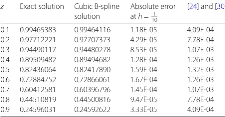
The precise solution isw(z) = (1 –z)ez. Algebraic outcomes for this problem are pre-sented in Table2forh=101 and Table3forh=15 respectively. The graphical comparison of absolute errors ath=101 andh=15 is demonstrated in Figs.1and2respectively.
At h= 101 we will have unknowns li where i= –1, 0, 1, . . . ,n+ 1. At n= 10 we will have seven equations from Eq. (12), three equations from Eq. (13), three equations from Eq. (14), so in total we will have thirteen equations and thirteen unknowns. The values of
Table 2 Algebraic outcomes for Problem1ath=101
z Exact solution Cubic B-spline
solution
Absolute error ath=101
[24] and [30]
0.1 0.99465383 0.99464116 1.18E-05 4.09E-04
0.2 0.97712221 0.97707373 4.29E-05 7.78E-04
0.3 0.94490117 0.94480278 8.53E-05 1.07E-03
0.4 0.89509482 0.89494682 1.28E-04 1.26E-03
0.5 0.82436064 0.82417890 1.59E-04 1.32E-03
0.6 0.72884752 0.72866061 1.67E-04 1.26E-03
0.7 0.60412581 0.60396796 1.45E-04 1.07E-03
0.8 0.44510819 0.44500816 9.47E-05 7.78E-04
0.9 0.24596031 0.24592622 3.33E-05 4.09E-04
Error*=Exact solution–Approximate solution
Table 3 Algebraic outcomes for Problem1ath=15
z Exact solution Cubic B-spline
solution
Absolute error ath=15
Pervaiz [1]
0.2 0.97712221 0.976933603 1.89E-04 1.21E-03
0.4 0.89509482 0.894500554 5.94E-04 1.97E-03
0.6 0.72884752 0.728081868 7.66E-04 2.17E-03
Figure 1Comparison of our method and [24] and [30] for Problem1
Figure 2Comparison of our method and [1] for Problem1
thirteen unknownsliwherei= –1, 0, 1, . . . , 11 are
l–1= 0.330000000000000, l0= 1.001666666666667,
l1= 0.996666666666667, l2= 0.979513602244758,
l3= 0.947721275080079, l4= 0.898417972748468,
l5= 0.828287737175295, l6= 0.733504478738225,
l7= 0.609658034368616, l8= 0.451671157504189,
l9= 0.253706303989511, l10= 0.009060939428197,
l11= –0.289950061702298.
Table 4 The results of Problem1from [9]
z Exact solution Sinc-Galerkin
solution
Absolute relative error (ARE) 1.0×e–3
0.0414 0.99911 0.99911 0.0
0.3131 0.93944 0.93943 0.01
0.5 0.82436 0.82432 0.03
0.6868 0.62243 0.62239 0.07
0.8278 0.39404 0.39400 0.09
0.9585 0.10822 0.10821 0.10
Table 5 Estimated derivative at the knots for Problem1
z Exactw(1)(z) Cubic B-spline
w(1)(z)
Absolute error ofw(1)(z)
Exactw(2)(z) Cubic B-spline
w(2)(z)
Absolute error ofw(2)(z)
0.1 –0.110517092 –0.11074035 2.23E-04 –1.21568801 –1.214807005 8.81E-04
0.2 –0.244280552 –0.244660538 3.80E-04 –1.46568331 –1.463596755 2.09E-03
0.3 –0.404957642 –0.405399753 4.42E-04 –1.75481645 –1.751187536 3.63E-03
0.4 –0.596729879 –0.59711663 3.87E-04 –2.088554577 –2.083150017 5.40E-03
0.5 –0.824360635 –0.824568788 2.08E-04 –2.473081906 –2.465893125 7.19E-03
0.6 –1.09327128 –1.093201278 7.00E-05 –2.915390081 –2.906756682 8.63E-03
0.7 –1.409626895 –1.40924466 3.82E-04 –3.423379603 –3.414110953 9.27E-03
0.8 –1.780432743 –1.779823367 6.09E-04 –4.005973671 –3.997463193 8.51E-03
0.9 –2.2136428 –2.213075086 5.68E-04 –4.673245911 –4.66757119 5.67E-03
liwherei= –1, 0, 1, . . . , 6 are
l–1= 0.986666666666667, l0= 1.001666666666667,
l1= 0.986666666666667, l2= 0.908268286018834,
l3= 0.747263518996417, l4= 0.471168850266235,
l5= 0.036243757712787, l6= –0.616143881117384.
The results of [9] for Problem1is demonstrated as follows in Table4, and obviously our results are encouraging.
Solving with cubic B-spline method, we also can acquire the estimated derivative at the knots, which is described in Table5, which is the main advantage of cubic B-spline method, as other methods are unable to obtain these values.
Problem 2
w(6)(z) +zw(z) = –24 + 11z+ (z)3 ez, 0≤z≤1,
subject to
w(0) = 0, w(1) = 0, w(0) = 1, w(1) = –e,
w(0) = 0, w(1) = –4e.
The exact solution isw(z) =z(1 –z)ez. Algebraic outcomes for this problem are pre-sented in Table6forh= 1
10 and Table7forh= 1
Table 6 Algebraic outcomes for Problem2ath=101
z Exact solution Cubic B-spline
solution
Absolute error ath=101
0.1 0.099465383 0.099427251 3.81E-05
0.2 0.195424441 0.195265639 1.59E-04
0.3 0.283470350 0.283129607 3.41E-04
0.4 0.358037927 0.357504923 5.33E-04
0.5 0.412180318 0.411506700 6.74E-04
0.6 0.437308512 0.436600310 7.08E-04
0.7 0.422888069 0.422279569 6.08E-04
0.8 0.356086549 0.355695711 3.91E-04
0.9 0.221364280 0.221229780 1.35E-04
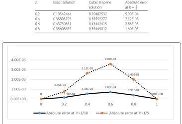
Table 7 Algebraic outcomes for Problem2ath=15
z Exact solution Cubic B-spline
solution
Absolute error ath=15
0.2 0.19542444 0.19482537 5.99E-04
0.4 0.35803793 0.35592277 2.12E-03
0.6 0.43730851 0.43442415 2.88E-03
0.8 0.35608655 0.35449012 1.60E-03
Figure 3Comparison of exact and cubic-B solution for Problem2
At h= 101 we will have unknowns li where i= –1, 0, 1, . . . ,n+ 1. At n= 10 we will have seven equations from Eq. (12), three equations from Eq. (13), three equations from Eq. (14), so in total we will have thirteen equations and thirteen unknowns. The values of thirteen unknownsliwherei= –1, 0, 1, . . . , 11 are
l–1= –0.100000000000, l0= 0, l1= 0.100000000000,
l2= 0.196563506057683, l3= 0.285339812568966,
l4= 0.360854884390805, l5= 0.416270189387388,
l6= 0.443104558445803, l7= 0.430913439191555,
l8= 0.366919100583079, l9= 0.235584425133117,
Table 8 The maximum absolute errors of Problem2from [30]
N Second order
method
7 2.99×10⁻²
15 7.00×10⁻³
31 1.80×10⁻³
Table 9 Estimated derivative at the knots for Problem2
z Exactw(1)(z) Cubic B-spline
w(1)(z)
Absolute error ofw(1)(z)
Exactw(2)(z) Cubic B-spline
w(2)(z)
Absolute error ofw(2)(z)
0.1 0.983602117 0.98281753 7.85E-04 –0.342603 –0.343649394 1.05E-03
0.2 0.928266096 0.926699063 1.57E-03 –0.781698 –0.778719955 2.98E-03
0.3 0.823413873 0.821456892 1.96E-03 –1.336360 –1.326123469 1.02E-02
0.4 0.656402867 0.654651884 1.75E-03 –2.028882 –2.009976683 1.89E-02
0.5 0.412180318 0.41124837 9.32E-04 –2.885262 –2.858093594 2.72E-02
0.6 0.072884752 0.073216249 3.31E-04 –3.935777 –3.902548831 3.32E-02
0.7 –0.382613014 –0.380927289 1.69E-03 –5.215620 –5.180321935 3.53E-02
0.8 –0.979238009 –0.97664507 2.59E-03 –6.765644 –6.734033684 3.16E-02
0.9 –1.746318209 –1.743986109 2.33E-03 –8.633207 –8.612787083 2.04E-02
Ath=1
5 we will have unknownsliwherei= –1, 0, 1, . . . ,n+ 1. Atn= 5 we will have two equations from Eq. (12), three equations from Eq. (13), three equations from Eq. (14), so in total we will have eight equations and eight unknowns. The values of eight unknowns
liwherei= –1, 0, 1, . . . , 6 are
l= –0.2000000002806, l0= –0.0000000002242,
l1= 0.2000000015886, l2= 0.3689521916188,
l3= 0.4597278365167, l4= 0.3986813363644,
l5= 0.0724875152029, l6= –0.6886313967683.
The maximum absolute errors corresponding to Problem2in [30] are demonstrated in Table8, and obviously our results are encouraging.
Solving with cubic B-spline method, we also can acquire the estimated derivative at the knots, which is described in Table9, which is the main advantage of cubic B-spline method, as other methods are unable to obtain these values.
Problem 3
w(6)(z) +e–zw(z) = –720 +z– (z)2 3e–z, 0≤z≤1,
subject to
w(0) = 0, w(1) = 0, w(0) = 0, w(1) = 0, w(0) = 0, w(1) = 0.
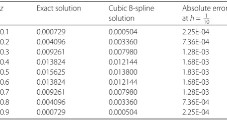
The exact solution isw(z) = (z)3(1 –z)3. Algebraic outcomes for this problem are pre-sented in Table10forh=101 and Table11forh=15respectively. The graphical comparison of absolute errors ath=101 andh=15 is demonstrated in Fig.4.
Table 10 Algebraic outcomes for Problem3ath=101
z Exact solution Cubic B-spline
solution
Absolute error ath=101
0.1 0.000729 0.000504 2.25E-04
0.2 0.004096 0.003360 7.36E-04
0.3 0.009261 0.007980 1.28E-03
0.4 0.013824 0.012144 1.68E-03
0.5 0.015625 0.013800 1.83E-03
0.6 0.013824 0.012144 1.68E-03
0.7 0.009261 0.007980 1.28E-03
0.8 0.004096 0.003360 7.36E-04
0.9 0.000729 0.000504 2.25E-04
Table 11 Algebraic outcomes for Problem3ath=15
z Exact solution Cubic B-spline
solution
Absolute error ath=15
0.2 0.004096 0.001536 2.56E-03
0.4 0.013824 0.007680 6.14E-03
0.6 0.013824 0.007680 6.14E-03
0.8 0.004096 0.001536 2.56E-03
Figure 4Comparison of exact and cubic-B solution for Problem3
Eq. (14), so in total we will have thirteen equations and thirteen unknowns. The values of thirteen unknownsliwherei= –1, 0, 1, . . . , 11 are
l–1= 0, l0= 0, l1= 0, l2= 0.003023996050353,
l3= 0.008063989424737, l4= 0.012599983512128,
l5= 0.014399981311357, l6= 0.012599983874666,
l7= 0.008063989877409, l8= 0.003023996294690,
l9= 0, l10= 0, l11= 0.
Ath=1
Table 12 The maximum absolute errors of Problem3from [9]
z Exact solution Sinc-Galerkin
solution
Absolute relative error (ARE) 1.0e–3
0.2764 0.008000 0.008997 0.32
0.4205 0.014469 0.014465 0.26
0.5 0.015625 0.015620 0.25
0.6550 0.011539 0.011536 0.28
0.8324 0.002715 0.002714 0.45
Table 13 Estimated derivative at the knots for Problem3
z Exactw(1)(z) Cubic B-spline
w(1)(z)
Absolute error ofw(1)(z)
Exactw(2)(z) Cubic B-spline
w(2)(z)
Absolute error ofw(2)(z)
0.1 0.01944 0.01511998 4.32E-03 0.297 0.302399605 5.40E-03
0.2 0.04608 0.040319947 5.76E-03 0.192 0.201599732 9.60E-03
0.3 0.05292 0.047879937 5.04E-03 –0.063 –0.050399929 1.26E-02
0.4 0.03456 0.031679959 2.88E-03 –0.288 –0.273599629 1.44E-02
0.5 0 1.81884E-09 1.82E-09 –0.375 –0.359999523 1.50E-02
0.6 –0.03456 –0.031679957 2.88E-03 –0.288 –0.273599656 1.44E-02
0.7 –0.05292 –0.047879938 5.04E-03 –0.063 –0.050399959 1.26E-02
0.8 –0.04608 –0.040319949 5.76E-03 0.192 0.201599729 9.60E-03
0.9 –0.01944 –0.015119981 4.32E-03 0.297 0.302399629 5.40E-03
liwherei= –1, 0, 1, . . . , 6 are
l–1= 0, l0= 0, l1= 0, l2= 0.009215951379013,
l3= 0.009215952744138, l4= 0, l5= 0, l6= 0.
The results of [9] for Problem3are demonstrated in Table12and obviously our results are encouraging.
Solving with Cubic B-spline method, we also can acquire the estimated derivative at the knots, which is described in Table13, which is the main advantage of cubic B-spline method, as other methods are unable to obtain these values.
Problem 4
w(6)(z) =Cos(z) –Sin(z), 0≤z≤1,
subject to
w(0) = 1, w(1) =Cos(1) +Sin(1), w(0) = 1, w(1) =Cos(1) –Sin(1),
w(0) = –1, w(1) = –Cos(1) –Sin(1).
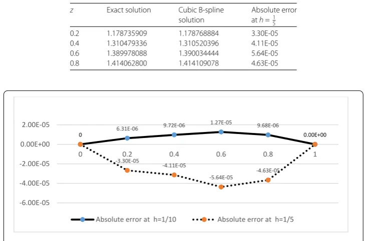
The precise solution isw(z) =Cos(z) +Sin(z). Algebraic outcomes for this problem are presented in Table14forh=101 and Table15forh=15 respectively. The graphical com-parison of absolute errors ath=101 andh=15is demonstrated in Fig.5.
Table 14 Algebraic outcomes for Problem4ath=101
z Exact solution Cubic B-spline
solution
Absolute error ath=101
0.1 1.094837582 1.094840345 2.76E-06
0.2 1.178735909 1.178742216 6.31E-06
0.3 1.250856696 1.250865071 8.38E-06
0.4 1.310479336 1.310489051 9.72E-06
0.5 1.357008100 1.357019339 1.12E-05
0.6 1.389978088 1.389990786 1.27E-05
0.7 1.409059875 1.409072555 1.27E-05
0.8 1.414062800 1.414072477 9.68E-06
0.9 1.404936878 1.404940836 3.96E-06
Table 15 Algebraic outcomes for Problem4ath=15
z Exact solution Cubic B-spline
solution
Absolute error ath=15
0.2 1.178735909 1.178768884 3.30E-05
0.4 1.310479336 1.310520396 4.11E-05
0.6 1.389978088 1.390034444 5.64E-05
0.8 1.414062800 1.414109078 4.63E-05
Figure 5Comparison of exact and cubic-B solution for Problem4
thirteen unknownsliwherei= –1, 0, 1, . . . , 11 are
l–1= 0.896666666666667, l0= 1.001666666666667,
l1= 1.096666666666667, l2= 1.180708735596316,
l3= 1.252951688415917, l4= 1.312674935541193,
l5= 1.359282877916855, l6= 1.392309586646931,
l7= 1.411423490072131, l8= 1.416431780494556,
l9= 1.407284247601092, l10= 1.384076246160497,
l11= 1.347050511813141.
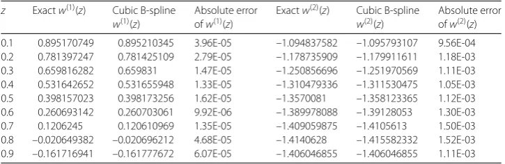
Table 16 Estimated derivative at the knots for Problem4
z Exactw(1)(z) Cubic B-spline
w(1)(z)
Absolute error ofw(1)(z)
Exactw(2)(z) Cubic B-spline
w(2)(z)
Absolute error ofw(2)(z)
0.1 0.895170749 0.895210345 3.96E-05 –1.094837582 –1.095793107 9.56E-04
0.2 0.781397247 0.781425109 2.79E-05 –1.178735909 –1.179911611 1.18E-03
0.3 0.659816282 0.659831 1.47E-05 –1.250856696 –1.251970569 1.11E-03
0.4 0.531642652 0.531655948 1.33E-05 –1.310479336 –1.311530475 1.05E-03
0.5 0.398157023 0.398173256 1.62E-05 –1.3570081 –1.358123365 1.12E-03
0.6 0.260693142 0.260703061 9.92E-06 –1.389978088 –1.39128053 1.30E-03
0.7 0.1206245 0.120610969 1.35E-05 –1.409059875 –1.4105613 1.50E-03
0.8 –0.020649382 –0.020696212 4.68E-05 –1.4140628 –1.415582332 1.52E-03
0.9 –0.161716941 –0.161777672 6.07E-05 –1.406046855 –1.406046855 1.11E-03
in total we will have eight equations and eight unknowns. The values of eight unknowns
liwherei= –1, 0, 1, . . . , 6 are as follows.
Solving with cubic B-spline method, we also can acquire the estimated derivative at the knots, which is described in Table16, which is the main advantage of cubic B-spline method, as other methods are unable to obtain these values.
4 Conclusion
The preceding segments demonstrate that the cubic B-spline technique is a sensible tac-tic to the numerical solution of sixth order BVP. The calculations associated with the examples deliberated above were accomplished by using Matlab R2015a. The algebraic outcomes validate the effectiveness and accurateness of the anticipated scheme. The an-ticipated algorithm formed a rapidly convergent series. We recommend that the cubic B-spline technique can also be accommodating when we investigate further higher order BVPs. It works soundly for higher order problems and signifies the fastest convergence as well as a notably low error.
Acknowledgements
The authors are very thankful to the reviewer for comments and suggestions, and this work was supported by the last author’s (S. Jain) research grant under the SERB Project Number: MTR/2017/000194.
Funding Not applicable.
Availability of data and materials None.
Competing interests
The authors declare that they have no competing interests.
Authors’ contributions
All authors contributed equally. All authors read and approved the final manuscript.
Author details
1Department of Mathematics, Government College Women University, Faisalabad, Pakistan.2Department of
Mathematics, Government College University, Faisalabad, Pakistan.3Department of Mathematics, Anand International College of Engineering, Jaipur, India.4International Centre for Basic and Applied Sciences, Jaipur, India.5Department of Mathematical Science, BUITEMS, Quetta, Pakistan.6Department of Mathematics, Division of Science and Technology, University of Education, Lahore, Pakistan.7Department of Mathematics, Poornima College of Engineering, Jaipur, India.
Publisher’s Note
Springer Nature remains neutral with regard to jurisdictional claims in published maps and institutional affiliations.
References
1. Baldwin, P.: Asymptotic estimates of the eigenvalues of a sixth-order boundary-value problem obtained by using global phase-integral methods. Philos. Trans. R. Soc. Lond. A, Math. Phys. Eng. Sci.322(1566), 281–305 (1987) 2. Boutayeb, A., Twizell, E.: Numerical methods for the solution of special sixth-order boundary-value problems. Int. J.
Comput. Math.45(3–4), 207–223 (1992)
3. Caglar, H., Caglar, N., Elfaituri, K.: B-spline interpolation compared with finite difference, finite element and finite volume methods which applied to two-point boundary value problems. Appl. Math. Comput.175(1), 72–79 (2006) 4. Chandrasekhar, S.: Hydrodynamic and Hydromagnetic Stability. Dover, New York (2013)
5. Chawla, M., Katti, C.: Finite difference methods for two-point boundary value problems involving high order differential equations. BIT Numer. Math.19(1), 27–33 (1979)
6. Dehghan, M., Lakestani, M.: Numerical solution of nonlinear system of second-order boundary value problems using cubic B-spline scaling functions. Int. J. Comput. Math.85(9), 1455–1461 (2008)
7. Ejaz, S.T., Mustafa, G., Khan, F.: Subdivision schemes based collocation algorithms for solution of fourth order boundary value problems. Math. Probl. Eng.2015, Article ID 240138 (2015)
8. El-Gamel, M., Cannon, J., Zayed, A.: Sinc-Galerkin method for solving linear sixth-order boundary-value problems. Math. Comput.73(247), 1325–1343 (2004)
9. Glatzmaier, G.A.: Numerical simulations of stellar convective dynamos III. At the base of the convection zone. Geophys. Astrophys. Fluid Dyn.31(1–2), 137–150 (1985)
10. Gupta, Y., Kumar, M.: B-spline method for solution of linear fourth order boundary value problem. Can. J. Comput. Math. Nat. Sci. Eng. Med.2(7), 166–169 (2011)
11. Hakeem, A., Rehman, S., Pervaiz, A., Iqbal, M.: Non-polynomial cubic spline approach for numerical approximation of second order linear Klein–Gordon equation. Pak. J. Sci.67(4), 377–382 (2015)
12. He, J.-H.: Variational approach to the sixth-order boundary value problems. Appl. Math. Comput.143(2), 537–538 (2003)
13. Kanwal, G., Ghaffar, A., Hafeezullah, M.M., Manan, S.A., Rizwan, M., Rahman, G.: Numerical solution of 2-point boundary value problem by subdivision scheme. Commun. Math. Appl.10(1), 19–29 (2019)
14. Khalid, A, Naeem, M.N.: Cubic B-spline solution of nonlinear sixth order boundary value problems. Punjab Univ. J. Math.50(4), 91–103 (2018)
15. Khan, A., Sultana, T.: Parametric quintic spline solution for sixth order two point boundary value problems. Filomat
26(6), 1233–1245 (2012)
16. Kumar, M., Gupta, Y.: Methods for solving singular boundary value problems using splines: a review. J. Appl. Math. Comput.32(1), 265–278 (2010)
17. Lang, F.-G., Xu, X.-P.: A new cubic B-spline method for linear fifth order boundary value problems. J. Appl. Math. Comput.36(1), 101–116 (2011)
18. Loghmani, G., Ahmadinia, M.: Numerical solution of sixth order boundary value problems with sixth degree B-spline functions. Appl. Math. Comput.186(2), 992–999 (2007)
19. Lucas, T.R.: Error bounds for interpolating cubic splines under various end conditions. SIAM J. Numer. Anal.11(3), 569–584 (1974)
20. Manan, S.A., Ghaffar, A., Rizwan, M., Rahman, G., Kanwal, G.: A subdivision approach to the approximate solution of 3rd order boundary value problem. Commun. Math. Appl.9(4), 499–512 (2018)
21. Mustafa, G., Abbas, M., Ejaz, S.T., Ismail, A.I.M., Khan, F.: A numerical approach based on subdivision schemes for solving non-linear fourth order boundary value problems. J. Comput. Anal. Appl.23(4), 607–623 (2017) 22. Mustafa, G., Ejaz, S.T.: Numerical solution of two-point boundary value problems by interpolating subdivision
schemes. Abstr. Appl. Anal.2014, Article ID 721314 (2014)
23. Noor, M.A., Mohyud-Din, S.T.: Variational iteration technique for solving linear and nonlinear sixth order boundary value problems. Int. J. Comput. Appl. Math.2, 163–172 (2007)
24. Noor, M.A., Mohyud-Din, S.T.: Homotopy perturbation method for solving sixth-order boundary value problems. Comput. Math. Appl.55(12), 2953–2972 (2008)
25. Noor, M.A., Noor, K.I., Mohyud-Din, S.T.: Variational iteration method for solving sixth-order boundary value problems. Commun. Nonlinear Sci. Numer. Simul.14(6), 2571–2580 (2009)
26. Pervaiz, A., Ahmad, A., Zafar, Z., Ahmad, M.: Numerical solution of sixth order BVPs by applying non-polynomial spline method. Pak. J. Sci.66(2), 110–116 (2014)
27. Schalkoff, R.J.: Artificial Neural Networks, vol. 1. McGraw-Hill, New York (1997)
28. Siddiqi, S.S., Akram, G.: Septic spline solutions of sixth-order boundary value problems. J. Comput. Appl. Math.215(1), 288–301 (2008)
29. Siddiqi, S.S., Akram, G., Nazeer, S.: Quintic spline solution of linear sixth-order boundary value problems. Appl. Math. Comput.189(1), 887–892 (2007)
30. Tirmizi, I.A., Khan, M.A.: Non-polynomial splines approach to the solution of sixth-order boundary-value problems. Appl. Math. Comput.195(1), 270–284 (2008)
31. Toomre, J., Zahn, J.-P., Latour, J., Spiegel, E.: Stellar convection theory. II—Single-mode study of the second convection zone in an A-type star. Astrophys. J.207, 545–563 (1976)
32. Twizell, E.: Numerical methods for sixth-order boundary value problems. In: Numerical Mathematics Singapore 1988, pp. 495–506. Springer, Berlin (1988)
33. Twizell, E., Boutayeb, A.: Numerical methods for the solution of special and general sixth-order boundary-value problems, with applications to Benard layer eigenvalue problems. Proc. R. Soc. Lond., Ser. A, Math. Phys. Eng. Sci.431, 433–450 (1990)
34. Ullah, I., Khan, H., Rahim, M.T.: Numerical solutions of fifth and sixth order nonlinear boundary value problems by Daftardar Jafari method. J. Comput. Eng.2014, Article ID 286039 (2014)
![Figure 1 Comparison of our method and [24] and [30] for Problem 1](https://thumb-us.123doks.com/thumbv2/123dok_us/923316.1111912/8.595.115.480.81.239/figure-comparison-method-problem.webp)
![Table 4 The results of Problem 1 from [9]](https://thumb-us.123doks.com/thumbv2/123dok_us/923316.1111912/9.595.116.479.219.336/table-results-problem.webp)
![Table 8 The maximum absolute errors of Problem 2 from [30]](https://thumb-us.123doks.com/thumbv2/123dok_us/923316.1111912/11.595.254.339.100.153/table-maximum-absolute-errors-problem.webp)
![Table 12 The maximum absolute errors of Problem 3 from [9]](https://thumb-us.123doks.com/thumbv2/123dok_us/923316.1111912/13.595.115.479.211.328/table-maximum-absolute-errors-problem.webp)