R E S E A R C H
Open Access
Control optimization and homoclinic
bifurcation of a prey–predator model with
ratio-dependent
Zhenzhen Shi
1, Jianmei Wang
1, Qingjian Li
2and Huidong Cheng
1**Correspondence:
[email protected] 1College of Mathematics and
Systems Science, Shandong University of Science and Technology, Qingdao, China Full list of author information is available at the end of the article
Abstract
In this paper, a predator–prey model with ratio-dependent and impulsive state feedback control is constructed, where the pest growth rate is related to an Allee effect. Firstly, the existence condition of the homoclinic cycle is obtained by analyzing the control parameterq. The existence, uniqueness and asymptotic stability of the periodic orbit are discussed by using the geometric theory of the differential equations, the method of successor functions and analog of the Poincaré criterion. Secondly, we formulate a control optimization with a minimal total cost in pest management, and we obtain an optimal economic threshold. Finally, we verify the main results by numerical simulation.
MSC: 34C25; 34D20; 92B05; 34A37
Keywords: Semi-continuous dynamic systems; Order one periodic orbit; Homoclinic cycle; Subsequence functions; Optimization
1 Introduction
Differential equations can be applied extensively in many fields, including economic de-velopment, environmental protection, population ecology, infectious diseases and phar-macokinetics, and the cultivation of micro-organisms [1–6]. In [3], Cuiet al.proposed the fractional differential equations and analyzed the uniqueness of solution for boundary value problems. Many researchers have obtained very good achievements in the field of stochastic differential equations [7–12].
In recent decades, many researchers have found that the occurrence of some biological phenomena and the optimal control of some life phenomena were not continuous pro-cesses, but the transient behavior of an impulse, so we should use impulsive differential equations to describe these phenomena. The theory of impulsive differential equations is proposed on the basis of continuous differential equation theory, which is difficult but valuable. It is widely applied in the harvest description [13–16], ecological resources [17–
26], pest control [27–31] and epidemiologic control [32–36]. Many scholars investigated state-dependent pulse differential equations in predator–prey model to simulate the pest management including the periodic release of natural enemies [37–39] and the periodic release of natural enemies combined with periodic spraying of pesticides [40–46]. On the
other hand, the bifurcation theory has been widely applied in the continuous dynamic system [47–49]. However, its application in impulsive dynamical system was little.
In [50], Zhanget al.proposed a predator–prey model with multi-state pulse feedback control as follows:
whereh1andh2are the biological control level (i.e.the threshold with slight damage to the
crops) and the chemical control level (i.e.pest economic injury threshold), respectively.
yMLrepresents the predator maintainable level atx=h1. It is interesting and practically
significant to involve chemical and biological controls at different economic thresholds, but there is a key problem to be identified in the model. Biological control can be adopted atx=h1andy<yML, but for a higher pest densityx=h, whereh1<h<h2, there no control
strategy is adopted, therefore the model is not flawless.
Based on above the factors, we propose a ratio-dependent predator–prey system with an integrated control strategy as follows:
⎧
of the prey and predator at timet1, respectively.rdenotes the intrinsic rate growth of
pests.h∈[h1,h2] represents the threshold of pests, whereh1andh2are biological control level and chemical control level, respectively.K> 0 represents the environment carrying capacity of pests.mdenotes the attack rate of predator.bdenotes the handling time of a single pest by natural enemies.cis the conversion ratio of consumed pests into viable natural enemy offspring.β1is the death rate of predator. The parameterα1represents the
survival threshold of the pest population for the Allee effect. 0 <α1<K is the survival
threshold of the pest population for the strong Allee effect, –K <α1< 0 is the survival
threshold of the pest population for the weak Allee effect. In this paper, only 0 <α1<Kis
taken into consideration. For reducing the parameters, we nondimensionalize system (2) with the following scaling:
x1 K =x,
mby1
then the following form can be obtained:
The organizational structure of this article is as follows. In Sect.2, the existence of ho-mocilinic cycle and existence, uniqueness and asymptotic stability of the periodic orbit of system (3) are proved. Furthermore, the optimization problem is formulated to reduce the total cost of pest control (i.e.the predator and the spraying agent). In Sect.3, the nu-merical simulation of the concrete model is gradually carried out to verify the theoretical results. The final conclusion is drawn in Sect.4.
2 Dynamical analysis of system (3) 2.1 Equilibria
Without impulse effect, system (3) becomes the following:
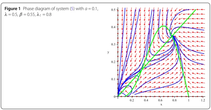
Figure 1Phase diagram of system (5) witha= 0.1,
λ= 0.5,β= 0.55,λ1= 0.8
2.2 Existence of the order one periodic orbit and homoclinic cycle of system (3)
By using the geometric theory of differential equations and the method of successor func-tion, the existence of the order one periodic orbit and homoclinic cycle of system (3) is investigated in this section. For the actual biological significance, we always suppose that
max{1+α– (1–α) 2–4λ(1–β
λ1)
2 ,h1}< (1 –p)h<h<min{
1+α+ (1–α)2–4λ(1–β λ1)
2 ,h2} and conditions
(H4), (H5) hold in the paper.
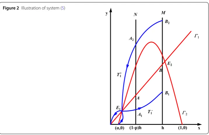
SetM={(x,y)|x=h, 0≤y≤yh}is called an impulsive set and setN={(x,y)|x= (1 – p)h,τ≤y≤(1 –q)yh+τ}is called a phase set. For convenience, for any pointL, letxLand yLdenote its abscissa and ordinate, respectively.Iis a continuous mapping which satisfies I(M) =Nand which is called an impulsive function. IfL(h,yL)∈M, then the impulse
func-tion transfers the pointLintoL+. We denote functionF(J) =J–as the trajectory starting
from the pointJ∈Nhits the impulse setMat the pointJ–. In this paper, the tendency of
trajectory is assumed to start from phase set. The unstable manifold and stable manifold of
E1are denoted asT1–(t,E1) andT1+(t,E1), respectively. At timet,T1–(t,E1) intersects phase
setN at pointA1 and impulsive setMat pointB1. At timet,T1+(t,E1) intersects phase
set N at pointA2 and impulsive setMat pointB2. IsoclineΓ1: dydt = 0 intersects phase
setNat pointAand impulsive setMat pointB, whereyA=h(1–p)(βλ1–β) andyB=
(λ1–β)h
β .
The functionϕ(y,q) = (1 –q)y+τis monotonically decreasing aboutq, and monotonically increasing abouty, thus there must exist a valueq∗∈(0, 1) such that pointBjumps toA
after the impulse effect,i.e.ϕ(yB,q∗) = (1 –q∗)yB+τ=yA, we haveq∗=p+(λ1βτ–β)h, for
con-venience, we setδ=p+(λβτ
1–β)h. For anyq∈(0, 1), the existence of order one periodic orbit
of system (3) is to be proved in the cases of 0 <q≤δandδ<q< 1, respectively (see Fig.2).
Case I0 <q≤δ.
Theorem 2.2
(a) If conditions(H4)(H5)andq=δhold,then system(3)admits a unique order one
periodic orbit.
(b) If conditions(H4)(H5)and0 <q∗<q<q0<δ< 1hold,then system(3)admits a
unique order one periodic orbit.
Proof The trajectory starting from the pointA∈Nhits the pointB∈M, then pointB∈M
Figure 2Illustration of system (5)
(a) Firstly, we prove the existence of the order one periodic orbit of system (3) in the case ofq=δ. In this case,B+coincides with point A, that is,AB andBAconstitute the order one periodic orbit.
(b) In this case,B+is aboveA. According to the impulsive equations of system (3), there
surely has a valueq∗∈(0,δ) satisfyingϕ(yB1,q∗) = (1 –q∗)yB1+τ =yA2, that is, pointB1 jumps to pointA2after impulse effect, also, there surely has a valueq0∈(q∗,δ) satisfying
ϕ(yB1,q
0) = (1 –q0)y
B1+τ =yA. For anyq∈(q∗,q
0), pointB
1jumps to pointB+1 after
im-pulsive effect, we have (1 –q0)y
B1 +τ =yA< (1 –q)yB1+τ =yB+1 < (1 –q
∗)y
B1 +τ =yA2, that is, yA<yB+1 <yA2. There must exist a trajectory going through point B
+
1 and
inter-secting the linex=hat pointC1, andI(C1) =C+1. In view of the disjointness of any two
trajectories and the vector field of system (3), we haveyB1<yC1<yB, (1 –q)yB1+τ=yB+1 < (1 –q)yC1+τ=yC+1, that is,yC+1 >yB+1. Thus the successor function [54, Definition 3.3] of B+1:g(B+1) =yC+
1 –yB+1 > 0.
A pointC((1 –p)h,yA2–ε) is selected in setN, whereε> 0 is small enough, then pointC is fully close to pointA2. SetF(C) =C2∈M, we haveyC2>yB1 due to continuous depen-dence of the solution on initial value and time, andC2is close enough to pointB1. Thus
we haveyC+2 >yB+1, and pointC
+
2 is close enough to pointB+1, then we haveyC+2 <yC, that is,g(C) =yC2+–yC< 0. According to [54, Lemma 3.2, 3.3], there has a pointP∈(B+1,C)
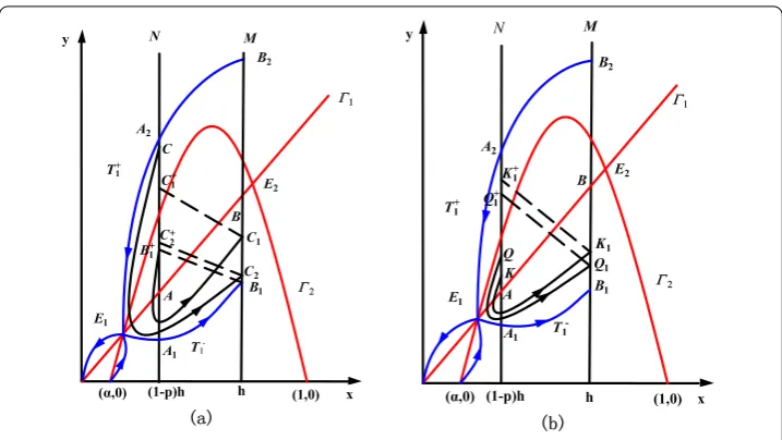
such thatg(P) = 0,i.e.system (3) admits the order one periodic orbit, whose initial point is between pointB+1 and pointCin the setN(see Fig.3(a)).
Next, we prove the uniqueness of the order one periodic orbit of system (3). We arbi-trarily select two pointsKandQin theAA2, whereyA<yK<yQ<yA2. SetF(K) =K1∈M,
F(Q) =Q1∈M, then we haveyQ1<yK1, andK1andQ1are, respectively, mapped toK1+∈N
andQ+1∈Nafter the impulse effect, then the successor functions ofK,Qsatisfy
g(K) –g(Q) = (yK1+–yK) – (yQ+1 –yQ)
Figure 3The existence and uniqueness of the order one periodic orbit of system (3) in case I. (a) The existence of the order one periodic solution of system (3). (b) The uniqueness of the order one periodic orbit of system (3)
= (yQ–yK) + (1 –q)yK1+τ– (1 –q)yQ1–τ
= (yQ–yK) + (1 –q)(yK1–yQ1) > 0.
Thus the successor function is monotonically increasing in theAA2, then there is only
one pointP∈(A,A2) such thatg(P) = 0, i.e.system (3) has only an order one periodic
orbit whenqsatisfies 0 <q<δ(see Fig.3(b)). This completes the proof.
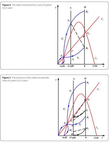
Theorem 2.3 If conditions(H4)and(H5)and q=q∗hold,then system(3)admits an order one homoclinic cycle;if q∈(0,q∗),system(3)does not admit an order one periodic orbit and the pests and natural enemy population will become extinct.
Proof Whenq=q∗, we haveϕ(yB1,q∗) = (1 –q∗)yB1+τ=yA2, then the closed curveB1A2∪
A2E1∪E1B1forms a cycle which passes through the saddleE1. Thus system (3) admits an
order one homoclinic cycle (see Fig.4).
Whenq∈(0,q∗), we have (1 –q)yB1+τ=yB+1 > (1 –q
∗)y
B1+τ =yA2 and the trajectory of system (3) starting fromB+1 will tend to origin whent→+∞, and it has no impulse
effect. Thus system (3) has no order one periodic orbit and the pest and natural enemy
population will become extinct. This completes the proof.
Case IIδ<q< 1.
Theorem 2.4 If the conditions(H4)(H5)andδ<q< 1hold,then the system(3)admits the order one periodic orbit.
Proof In this case, we know thatB+is belowA. SetF(B+) =S
1∈M, according to the
prop-erty of orbit of system (3), we knowyB>yS1, thus we haveyB+ >yS+
1, then the succes-sor function of pointB+isg(B+) =y
S+1 –yB+ < 0. A pointH((1 –p)h,ε)∈N is selected, whereε<τ, and setF(H) =H1∈M, after impulsive effect, pointH1 jumps toH1+, then yH+
Figure 4The order one homoclinic cycle of system (3) in case I
Figure 5The existence of the order one periodic orbit of system (3) in case II
Lemma 3.2, 3.3], there exists a point P∈(H,B+) satisfyingg(P) = 0, that is, system (3)
admits the order one periodic orbit, whose initial point is betweenHandB+in the setN.
This completes the proof (see Fig.5).
2.3 Stability of the order one periodic orbit of system (3)
Next, we study the stability of the order one periodic orbit of system (3).
Theorem 2.5 If conditions(H4), (H5),and(1 –α) + λαh– λ1αy1
(1+h)2 < 0and|χ|< 1hold,then
the order one periodic orbit of system(3)is orbitally asymptotically stable,where
χ=[(1 –p)h–α][1 – (1 –p)h](h+η1) (h–α)(1 –h)(h+η1) –λη1
For any point (x,y)∈Θ,α<x< 1 andy1<y<h, we have (1 –α) +λαh– λ1αy1
(1+h)2 < 0, so we can get
x(1 +α– 2x) + λxy (x+y)2 –
λ1xy
(x+y)2< (1 –α) +
λh
α – λ1αy1
(1 +h)2 < 0,
and due to|χ|< 1, we have
(1 –q)η1[(ξ0–α)(1 –ξ0) –ξλη0+0η0] η0[(ξ1–α)(1 –ξ1) –ξ1λη+η11]
< 1.
Therefore|μ2|< 1. According to the analog of the Poincaré criterion [55, Theorem 2.3],
we know that the order one periodic orbit of system (3) is orbitally asymptotically stable.
This completes the proof.
2.4 Determination of optimal pest economic threshold
In order to determine the optimum release amount of natural enemies and the optimal fre-quency of spraying chemical pesticide, we formulate the following optimization problem and find the optimal economic threshold.
Letl1represent the unit cost of the biological control,l2 the unit cost of the chemical
control. Our final purpose is to minimize the expenses of per unit period. We denote by
Fthe total expenses in a period of system (3), which is a function of the chemical control strengthp(h) and release amount of natural enemiesτ(h). Then we haveF(h) =l1τ(h) + l2p(h). Thus we formulate the following optimization model:
minF(h)
T(h)
s.t.h1<h<h2.
Solving the objective function yields the optimum economic thresholdh∗, which results in the optimum release amount of the predatorτ∗=τ(h∗), the optimal chemical control strengthp∗ =p(h∗) and the optimal control period of chemical controlT∗=T(τ∗,p∗). However, it is important to be noted that the optimal economic thresholdh∗is dependent on the ratio ofω=l2
l1.
3 Simulations and optimization
In order to verify the theoretical results obtained in this paper, a specific example is pre-sented in this section. Letα= 0.1,λ= 0.5,λ1= 0.8,β= 0.55,h1= 0.35,h2= 0.76,pmax= 0.3,
τmax= 0.1, τmin= 0.01,qmax= 0.8. By a simple calculation, the saddle point and locally
asymptotically stable point areE1(0.3349, 0.1522) andE0(0.7651, 0.3478), respectively. We
carry out simulations by changing the main parameterhand fixing all other parameters. The control parametersp,q,τ are calculated by (4).
3.1 Numerical simulations
Taking parametersα,λ,β,λ1into system (5), we can obtain ⎧
⎨ ⎩
dx
dt =x(t)[x(t) – 0.1][1 –x(t)] – 0.5x(t)y(t)
x(t)+y(t) , dy
dt = 0.8x(t)y(t)
x(t)+y(t) – 0.55y(t).
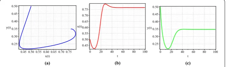
Figure 6Numerical simulations without impulsive. (a) Phase portrait ofx(t) andy(t). (b) Time series ofx(t). (c) Time series ofy(t)
Figure 7Numerical simulations in the case 0 <q<q∗. (a) Phase portrait ofx(t) andy(t). (b) Time series ofx(t). (c) Time series ofy(t)
Figure 8Numerical simulations in the caseq∗<q<δ. (a) Phase portrait ofx(t) andy(t). (b) Time series ofx(t). (c) Time series ofy(t)
Furthermore, Fig.6(a) shows the phase portrait ofx(t) andy(t), Fig.6(b) shows time series of x(t), Fig.6(c) shows time series of y(t). Letp= 0.27,h= 0.61,τ = 0.18, we shall get δ=p+(λβτ
1–β)h = 0.27 +
0.55×0.18
(0.8–0.55)×0.61= 0.92. Letq= 0.01 we shall get Fig.7. Figures7(a), 7(b) and7(c) show that system (3) does not have order one periodic orbit and the pest and natural enemy population become extinct when 0 <q<q∗. Letq= 0.6,q= 0.7 andq= 0.8 and we shall get a unique order one periodic solution and it is asymptotically stable (see Fig.8). Furthermore, according to Fig.8, we see that, as the parameterqincreases, the periodT becomes smaller. Figure9shows that system (3) admits the order one periodic orbit whenq>δ. According to Fig.9, we see that, as the parameterqincreases, the period
Figure 9Numerical simulations in the caseδ<q< 1. (a) Phase portrait ofx(t) andy(t). (b) Time series ofx(t). (c) Time series ofy(t)
Figure 10 Impulse periodTof the order one periodic solution varies with the economic thresholdh
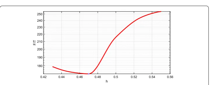
Figure 11 Cost per unit timeF/Ton the economic thresholdh
3.2 Optimum pest control level
The impulse periodT of the order one periodic orbit varies with the economic threshold
h, as is shown in Fig.10. And Fig.11shows the variation of cost per unit timeF/Tand the periodT with the pest control levelh. Assumel1= 10,000,l2= 100, we shall getω=ll21 =
1/100.
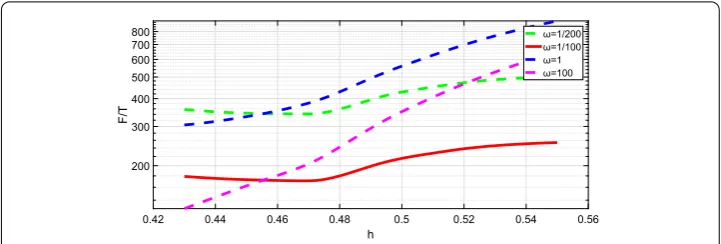
Figure 12 The change in the cost per unit timeF/Ton the economic thresholdhforω= 1/200, 1/100, 1, 100
4 Conclusion
In this paper, a predator–prey model with ratio-dependent and impulsive state feedback control is proposed. We take control measures that combine biological control and chem-ical control. The aim of this study is to get optimum pest control level and minimize the cost of pest control.
Based on the above analysis, both the predator and the prey are extinct when 0 <q<q∗, that is, the order one periodic orbit does not exist when 0 <q<q∗, system (3) admits an order one homoclinic cycle forq=q∗; we obtain a unique and stable order one periodic orbit according to the geometric theory of the differential equations and the method of subsequence functions in the case ofq∗<q<δ; and system (3) admits the order one peri-odic orbit in the case ofδ<q< 1.
In order to reduce the total cost of pest management, an optimization problem is formu-lated, and the optimal economic threshold and the minimum control cost are obtained. Finally, numerical simulation is carried out to verify the theoretical results.
Funding
The paper was supported by the National Natural Science Foundation of China (No. 11371230), Shandong Provincial Natural Science Foundation, China (No. S2015SF002), SDUST Research Fund (2014TDJH102), and Joint Innovative Center for Safe and Effective Mining Technology and Equipment of Coal Resources, Shandong Province of China.
Competing interests
The authors declare that they have no competing interests.
Authors’ contributions
All authors read and approved the final manuscript.
Author details
1College of Mathematics and Systems Science, Shandong University of Science and Technology, Qingdao, China.
2College of Foreign Languages, Shandong University of Science and Technology, Qingdao, China.
Publisher’s Note
Springer Nature remains neutral with regard to jurisdictional claims in published maps and institutional affiliations.
Received: 29 July 2018 Accepted: 13 December 2018
References
1. Bai, Z., Zhang, S., Sun, S., Yin, C.: Monotone iterative method for fractional differential equations. Electron. J. Differ. Equ.
2016, 6 (2016)
2. Liu, F.: Continuity and approximate differentiability of multisublinear fractional maximal functions. Math. Inequal. Appl.21(1), 25–40 (2018)
3. Cui, Y.: Uniqueness of solution for boundary value problems for fractional differential equations. Appl. Math. Lett.51, 48–54 (2016)
5. Lv, W., Wang, F.: Adaptive tracking control for a class of uncertain nonlinear systems with infinite number of actuator failures using neural networks. Adv. Differ. Equ.2017(1), 374 (2017)
6. Zou, Y., Liu, L., Cui, Y.: The existence of solutions for four-point coupled boundary value problems of fractional differential equations at resonance. Abstr. Appl. Anal.2014(13), 286 (2014)
7. Brauer, F., Soudack, A.C.: Stability regions in predator–prey systems with constant-rate prey harvesting. J. Math. Biol.
8(1), 55–71 (1979)
8. Yu, X., Yuan, S., Zhang, T.: Persistence and ergodicity of a stochastic single species model with Allee effect under regime switching. Commun. Nonlinear Sci. Numer. Simul.59, 359–374 (2018)
9. Liu, G., Wang, X., Meng, X.: Extinction and persistence in mean of a novel delay impulsive stochastic infected predator–prey system with jumps. Complexity2017(3), 115 (2017)
10. Zhang, T., Zhang, T., Meng, X.: Stability analysis of a chemostat model with maintenance energy. Appl. Math. Lett.68, 1–7 (2017)
11. Meng, X., Wang, L., Zhang, T.: Global dynamics analysis of a nonlinear impulsive stochastic chemostat system in a polluted environment. J. Appl. Anal. Comput.6(3), 865–875 (2016)
12. Zhao, Q., Li, X.: A Bargmann system and the involutive solutions associated with a new 4-order lattice hierarchy. Anal. Math. Phys.6(3), 237–254 (2016)
13. Wang, J., Cheng, H., Liu, H., Wang, Y.: Periodic solution and control optimization of a prey–predator model with two types of harvesting. Adv. Differ. Equ.2018(1), 41 (2018)
14. Wei, C., Chen, L.: Periodic solution and heteroclinic bifurcation in a predator–prey system with Allee effect and impulsive harvesting. Nonlinear Dyn.76(2), 1109–1117 (2014)
15. Martin, A., Ruan, S.: Predator–prey models with delay and prey harvesting. J. Math. Biol.43(3), 247–267 (2001) 16. Huang, M., Liu, S., Song, X., Chen, L.: Periodic solutions and homoclinic bifurcation of a predator–prey system with
two types of harvesting. Nonlinear Dyn.73(1–2), 815–826 (2013)
17. Zhao, L., Chen, L., Zhang, Q.: The geometrical analysis of a predator–prey model with two state impulses. Math. Biosci.
238(2), 55–64 (2012)
18. Tang, S., Chen, L.: Global attractivity in a food-limited population model with impulsive effects. J. Math. Anal. Appl.
292(1), 211–221 (2004)
19. Zhang, M., Song, G., Chen, L.: A state feedback impulse model for computer worm control. Nonlinear Dyn.85(3), 1–9 (2016)
20. Liu, H., Cheng, H.: Dynamic analysis of a prey–predator model with state-dependent control strategy and square root response function. Adv. Differ. Equ.2018(1), 63 (2018)
21. Jiang, G., Lu, Q.: Impulsive state feedback control of a predator–prey model. J. Comput. Appl. Math.200(1), 193–207 (2007)
22. Zhao, W., Li, J., Meng, X.: Dynamical analysis of SIR epidemic model with nonlinear pulse vaccination and lifelong immunity. Discrete Dyn. Nat. Soc.,2015, 848623 (2015)
23. Liu, X., Zhang, T., Meng, X., Zhang, T.: Turing-Hopf bifurcations in a predator–prey model with herd behavior, quadratic mortality and prey-taxis. Phys. A, Stat. Mech. Appl.496, 446–460 (2018)
24. Qi, H., Liu, L., Meng, X.: Dynamics of a nonautonomous stochastic SIS epidemic model with double epidemic hypothesis. Complexity2017(3), Article ID 4861391 (2017)
25. Li, Y., Cheng, H., Wang, Y.: A lycaon pictus impulsive state feedback control model with Allee effect and continuous time delay. Adv. Differ. Equ.2018(1), 367 (2018)
26. Zhang, T., Liu, X., Meng, X., Zhang, T.: Spatio-temporal dynamics near the steady state of a planktonic system. Comput. Math. Appl.75(12), 4490–4504 (2018)
27. Lenteren, J.C.: Integrated pest management in protected crops. Integr. Pest Manag. D17(3), 270–275 (1995) 28. Tian, Y., Zhang, T., Sun, K.: Dynamics analysis of a pest management prey–predator model by means of interval state
monitoring and control. Nonlinear Anal. Hybrid Syst.23, 122–141 (2017)
29. Wang, J., Cheng, H., Meng, X., Pradeep, B.S.A.: Geometrical analysis and control optimization of a predator–prey model with multi state-dependent impulse. Adv. Differ. Equ.2017(1), 252 (2017)
30. Pang, G., Chen, L.: Periodic solution of the system with impulsive state feedback control. Nonlinear Dyn.78(1), 743–753 (2014)
31. Chen, L.: Pest control and geometric theory of semi-continuous dynamical system. J. Beihua Univ. (2011). doi:1009-4822(2011)01-0001-09
32. Meng, X., Wang, L., Zhang, T.: Global dynamics analysis of a nonlinear impulsive stochastic chemostat system in a polluted environment. J. Appl. Anal. Comput.6(3), 865–875 (2016)
33. Miao, A., Wang, X., Zhang, T., Wang, W., Sampath Aruna Pradeep, B.: Dynamical analysis of a stochastic sis epidemic model with nonlinear incidence rate and double epidemic hypothesis. Adv. Differ. Equ.2017(1), 226 (2017) 34. Zhang, T., Ma, W., Meng, X.: Global dynamics of a delayed chemostat model with harvest by impulsive flocculant
input. Adv. Differ. Equ.2017(1), 115 (2017)
35. Lv, W., Wang, F., Li, Y.: Adaptive finite-time tracking control for nonlinear systems with unmodeled dynamics using neural networks. Adv. Differ. Equ.2018(1), 159 (2018)
36. Liu, F., Xue, Q.: Characterizations of the multiple Littlewood–Paley operators on product domains. Publ. Math. (Debr.)
92(3–4), 419–439 (2018)
37. Terry, A.J.: Biocontrol in an impulsive predator–prey model. Math. Biosci.256, 102–115 (2014)
38. Caltagirone, L.E., Doutt, R.L.: The history of the vedalia beetle importation to California and its impact on the development of biological control. Annu. Rev. Entomol.34(1), 1–16 (1989)
39. Xu, W., Chen, L., Chen, S., Pang, G.: An impulsive state feedback control model for releasing white-headed langurs in captive to the wild. Commun. Nonlinear Sci. Numer. Simul.34, 199–209 (2016)
40. Barclay, H.J.: Models for pest control using predator release, habitat management and pesticide release in combination. J. Appl. Ecol.19(2), 337–348 (1982)
41. Cheng, H., Wang, F., Zhang, T.: Multi-state dependent impulsive control for Holling I predator–prey model. Discrete Dyn. Nat. Soc.2012(12), Article ID 181752 (2012)
43. Huang, M., Song, X., Li, J.: Modelling and analysis of impulsive releases of sterile mosquitoes. J. Biol. Dyn.11(1), 147 (2017)
44. Wang, F., Zhang, X.: Adaptive finite time control of nonlinear systems under time-varying actuator failures. IEEE Trans. Syst. Man Cybern. Syst.https://doi.org/10.1109/TSMC.2018.2868329
45. Liu, F.: A note on Marcinkiewicz integrals associated to surfaces of revolution. J. Aust. Math. Soc.104(3), 380–402 (2018)
46. Wang, F., Chen, B., Sun, Y., Lin, C.: Finite time control of switched stochastic nonlinear systems. Fuzzy Sets Syst.
https://doi.org/10.1016/j.fss.2018.04.016
47. Huang, C., Cao, J., Xiao, M., Alsaedi, A., Alsaadi, F.E.: Controlling bifurcation in a delayed fractional predator–prey system with incommensurate orders. Appl. Math. Comput.293, 293–310 (2017)
48. Huang, C., Cao, J., Xiao, M., Alsaedi, A., Hayat, T.: Effects of time delays on stability and Hopf bifurcation in a fractional ring-structured network with arbitrary neurons. Commun. Nonlinear Sci. Numer. Simul.57, 1–13 (2018)
49. Cao, J., Guerrini, L., Cheng, Z.: Stability and Hopf bifurcation of controlled complex networks model with two delays. Appl. Math. Comput.343, 21–29 (2019)
50. Zhang, T., Meng, X., Liu, R., Zhang, T.: Periodic solution of a pest management Gompertz model with impulsive state feedback control. Nonlinear Dyn.78(2), 921–938 (2014)
51. Sen, M., Banerjee, M., Morozov, A.: Bifurcation analysis of a ratio-dependent predator–prey model with the Allee effect. Ecol. Complex.11(3), 12–27 (2012)
52. Xiao, D., Ruan, S.: Global dynamics of a ratio-dependent predator–prey system. J. Math. Biol.43(3), 268–290 (2001) 53. Sun, K., Zhang, T., Tian, Y.: Theoretical study and control optimization of an integrated pest management
predator–prey model with power growth rate. Math. Biosci.279, 13–26 (2016)
54. Liang, Z., Pang, G., Zeng, X., Liang, Y.: Qualitative analysis of a predator–prey system with mutual interference and impulsive state feedback control. Nonlinear Dyn.87(3), 1–15 (2016)