DOI: 10.1534/genetics.110.120311
Mapping Environment-Specific Quantitative Trait Loci
Xin Chen,* Fuping Zhao
†and Shizhong Xu
†,1*Department of Statistics and†Department of Botany and Plant Sciences, University of California, Riverside, California 92521
Manuscript received June 27, 2010 Accepted for publication August 21, 2010
ABSTRACT
Environment-specific quantitative trait loci (QTL) refer to QTL that express differently in different environments, a phenomenon called QTL-by-environment (Q3 E) interaction. Q3 Einteraction is a difficult problem extended from traditional QTL mapping. The mixture model maximum-likelihood method is commonly adopted for interval mapping of QTL, but the method is not optimal in handling QTL interacting with environments. We partitioned QTL effects into main and interaction effects. The main effects are represented by the means of QTL effects in all environments and the interaction effects are represented by the variances of the QTL effects across environments. We used the Markov chain Monte Carlo (MCMC) implemented Bayesian method to estimate both the main and the interaction effects. The residual error covariance matrix was modeled using the factor analytic covariance structure. A simulation study showed that the factor analytic structure is robust and can handle other structures as special cases. The method was also applied toQ3Einteraction mapping for the yield trait of barley. Eight markers showed significant main effects and 18 markers showed significantQ 3Einteraction. The 18 interacting markers were distributed across all seven chromosomes of the entire genome. Only 1 marker had both the main and theQ3Einteraction effects. Each of the other markers had either a main effect or aQ3Einteraction effect but not both.
G
ENOTYPE-BY-ENVIRONMENT (G 3 E) interac-tion is a very important phenomenon in quanti-tative genetics. With the advanced molecular technology and statistical methods for quantitative trait loci (QTL) mapping (Lander and Botstein 1989; Jansen 1993;Zeng1994), G3 E interaction analysis has shifted to
QTL-by-environment (Q3E) interaction. In the early stage of QTL mapping, almost all statistical methods were developed in a single environment (Paterson
et al. 1991; Stuber et al. 1992). Data from different
environments were analyzed separately and the con-clusions were drawn from the separate analyses of QTL across environments. These methods do not consider the correlation of data under different environments and thus may not extract maximum information from the data. Composite interval mapping for multiple traits can be used for Q 3 E interaction if different traits are treated as the same trait measured in different environments ( Jiangand Zeng 1995). This
multivar-iate composite interval mapping approach makes good use of all data simultaneously and increases statistical power of QTL detection and accuracy of the estimated QTL positions. However, the number of parameters of this method increases dramatically as the number of environments increases. Therefore, the method may
not be applied when the number of environments is large. Several other models have been proposed to solve the problem of a large number of environments ( Jansenet al.1995; Beavisand Keim1996; Romagosa
et al.1996). These methods were based on some special situations and assumptions. One typical assumption was independent errors or constant variances across envi-ronments. These assumptions are often violated in real QTL mapping experiments.
Earlier investigators realized the problem and adop-ted the mixed-model methodology to solve the problem (Piepho 2000; Boer et al. 2007). Under the
mixed-model framework, people can choose which mixed-model effects are random and which are fixed. The mixed-model methodology is very flexible, leading to an easy way to model genetic and environmental correlation between environments using a suitable error structure. Piepho(2000) proposed a mixed model to detect QTL
main effect across environments. Similar to the com-posite interval mapping analysis, his model incorpo-rated one putative QTL and a few cofactors. TheQ3E effects in the model were assumed to be random, which greatly reduced the number of estimated parameters. However, the fact that only one QTL is included in the model means that Piepho’s (2000) model remains a
single-QTL model rather than a multivariate model. Boeret al. (2007) proposed a step-by-step mixed-model
approach to detecting QTL main effects, Q 3 E in-teraction effects, and QTL responses to specific envi-ronmental covariates. In the final step, Boer et al.
1Corresponding author: Department of Botany and Plant Sciences,
University of California, Riverside, CA 92521. E-mail: [email protected]
(2007) rewrote the model to include all QTL in a multiple-QTL model and reestimated their effects.
In this study, we extended the Bayesian shrinkage method (Xu2003) to mapQ3Einteraction effects of
QTL. In the original study (Xu2003), we treated each
marker as a putative QTL and used the shrinkage method to simultaneously estimate marker effects of the entire genome. In the multiple-environment case, we can still use this approach to simultaneously evaluate marker effects under multiple environments but we can further partition the marker effects into main andQ3E interaction effects. For any particular marker, the mean of the marker effects represents the main effect and the variance of the marker effects represents the Q 3 E interaction effect for that marker. Under the Bayesian framework, we assigned a normal prior with zero mean and an unknown variance to each marker main effect and a multivariate normal prior with zero vector mean and homogeneous diagonal variance–covariance matrix to theQ3Einteraction effects of each maker. In multiple environments, the structure of the error terms might be very complicated since we need to consider the correla-tion of the same genotype under different environments. In our analysis, we used different variance–covariance structures to model the error terms. The simplest case was the homogeneous diagonal matrix, and the most complex choice was an unstructured matrix. We also used a heterogeneous diagonal matrix whose parame-ters are somewhere between the two models. Finally, we considered several factor analytic models. The reason to use the factor analytic structure is that it can separate genetic effects into common effects and environment-specific effects. In addition, the factor analytic structure is parsimonious and thus can sub-stantially reduce the computational burden of the mixed-model analyses.
THEORY AND METHOD
Hierarchical model: Letyj ¼ ½yj1yj2 . . . yjmT be an
m31 column vector for the observed phenotypic values of individual j measured from m environments for j¼1;. . .;n, where n is the sample size. Let qbe the number of QTL included in the model. The multivar-iate linear model is
yj¼b1 Xq
k¼1
Zjkgk1jj: ð1Þ
In the above model, b¼ ½b1b2 . . .bmT is an m31 vector for the intercepts. The dependent variableZjkis a genotype indicator variable for individualjat markerk and it is defined asZjk ¼ f 1;1gfor the two genotypes of a backcross (BC) individual orZjk ¼ f 1;0;1g for the three genotypes of an F2individual. The regression
coefficientgk¼ ½gk1gk2 . . .gkmT is an m31 vector of QTL effects for the m environments. Finally, jj ¼
½jj1jj2 . . . jjmTis anm31 vector for the residual errors. To model the Q 3 E interaction, we assume that gk follows a multivariate normal distribution,
pðgkÞ ¼Nðgkj1mak;Im3ms2kÞ; ð2Þ where 1m is a unity vector with dimensionm, Im3m is an m3midentity matrix,akis the mean value repre-senting the main QTL effect, andsk2is the variance ofg
k representing theQ3Einteraction. This type of model with further modeling on gk is called a hierarchical model. In the hierarchical model, the first moment parameterakis the main effect and the second moment parametersk2represents the degree ofQ 3E interac-tion. The residual error vector jj is assumed to be multivariate normal with density
pðjjÞ ¼Nðjjj0;QÞ; ð3Þ
whereQis anm3mvariance–covariance matrix, which can be chosen from a class of available forms (to be discussed later). We have now defined the data and parameters. The nest step of the Bayesian analysis is to choose the prior distribution and infer the posterior distribution for each parameter.
Prior distribution: We often have enough informa-tion from the data to estimate b and thus a flat (uninformative) prior was chosen for b; i.e., p(b)¼1. The main effect for thekth QTL was assigned the fol-lowing normal prior,
pðakÞ ¼Nðakj0;u2kÞ; ð4Þ where u2
k is the prior variance. A scaled inverse chi-square distribution was assigned tou2k, which is
pðu2
kÞ ¼Invx2ðuk2jt;vÞ: ð5Þ A special case of this prior is t¼v¼0, leading to pðu2
kÞ ¼1=u
2
k, called Jeffreys’ prior. However, as men-tioned byterBraaket al. (2005), this prior is improper
and leads to an improper posterior distribution. The revised prior is proposed by them and is claimed to lead to a proper posterior distribution. The revised prior is
pðu2
kÞ ¼Invx2ðu2kj 2d;0Þ; ð6Þ where 0,d #0.5. In this study we used the proper prior to avoid any potential problems caused by the improper posterior distribution. The same scaled inverse chi-square distribution was also assigned tosk2,
pðs2kÞ ¼Invx2ðs2kj 2d;0Þ: ð7Þ
Finally, we assumedQ¼Im3ms2, wheres2is a common residual variance and was assigned the same scaled inverse prior,
pðs2Þ ¼Invx2ðs2j 2d;0Þ: ð8Þ
Posterior distribution: The Markov chain Monte Carlo (MCMC) algorithm was used to implement the Bayesian shrinkage analysis. In the MCMC sampling, we need to derive only the fully conditional posterior distribution for each parameter. For example, the fully conditional posterior distribution forb is denoted by p(bj. . .), where the dots after the vertical bar represent the data and all other parameters. Except for the prior ofb, all other priors we chose in the previous section are conjugate. Therefore, the fully conditional posterior has the same form as the prior distribution. Derivation of the posterior distribution was not given and we simply provided the parameters of the fully conditional poste-rior distribution for each variable.
The posterior distribution forbis multivariate normal
pðbj . . .Þ ¼Nðbjmb;SbÞ; ð9Þ
where
mb ¼
1 n Xn j¼1 yj XQ k¼1 Zjkgk
!
ð10Þ
and
Sb¼1
nQ: ð11Þ
The posterior forgkis also multivariate normal,
pðgkj . . .Þ ¼Nðgkjmk;SkÞ; ð12Þ
where
mk¼ 1 s2
k
Im3m1
Xn
j¼1 ZTjkQ
1 Zjk
" #1
3 1
s2
k
Im3mak1
Xn
j¼1
ZTjkQ1ðyjb
Xq
k96¼kZjk9gk9Þ
" #
ð13Þ
and
Sk¼ 1
s2kIm3m1
Xn
j¼1
ZTjkQ1Z jk
" #1
: ð14Þ
The posterior distribution forakis normal,
pðakj . . .Þ ¼Nðakjzk;nkÞ; ð15Þ
where
zk¼ 1
u2k 1
m
s2k
11
s2k
Xm
i¼1
gki ð16Þ
and
nk¼ 1
u2k 1
m
s2k
1
: ð17Þ
We now discuss the posterior distributions for all the variance components,s2,s2k, andu2
kfork¼1,. . .,q. All of them are scaled inverse chi squares as given below,
pðs2
kj . . .Þ
¼Invx2 s2kjt1m;v1ðgk1makÞTðgk1makÞ
;
ð18Þ
pðu2kj Þ ¼Invx2ðu2kjt11;v1a2kÞ; ð19Þ
and
pðs2j . . .Þ ¼Invx2ðs2jt1nm;v1SSÞ; ð20Þ
where
SS¼X
n
j¼1
yjb Xq
k¼1 Zjkgk
!T
yjb Xq
k¼1 Zjkgk
!
:
ð21Þ
MCMC sampling: Since all the fully conditional posterior distributions have closed-form distributions, either a normal or a scaled inverse chi-square, Gibbs sampler was used for sampling all the variables, which is summarized below:
1. Initialize all variables by sampling the values from their prior distributions.
2. Sample the parameters sequentially from their cor-responding posterior distributions.
3. Repeat the sampling cycle until the chain reaches a desired length.
The posterior sample contains all the observations after burn-in deletion and chain thinning. Post-MCMC analysis was performed on the posterior sample. We often ran multiple chains and took the average poste-rior statistics across the chains as the Bayesian estimates of the parameters.
Covariance structure: We now introduce several alternative covariance structures for the residual errors. Identity matrix:The simple structure described earlier,
Q¼Ims2, is called the scaled identity matrix structure.
This assumption is oversimplified and should be relaxed in real data analysis.
Diagonal matrix:The covariance matrix is defined as
in most situations. Eachdwas assigned a scaled inverse chi-square distribution and the fully conditional poste-rior distribution fordiis
pðdij . . .Þ ¼Invx2ðdijt1n; v1SSiÞ; ð23Þ where
SSi¼ Xn
j¼1
yjibi Xq
k¼1 Zjkgki
!2
: ð24Þ
Unstructured matrix: The unstructured covariance matrix has been used before by Jiang and Zeng
(1995) for multivariate QTL mapping. The only restriction for matrixQis positive definite. We assigned
an inverse Wishart prior distribution toQ. This prior is the multivariate version of the scaled inverse chi-square distribution,
pðQÞ ¼Inv - WishartðQjt;vÞ; ð25Þ
wheret.m1 is the prior degree of belief andv.0 is a positive definite matrix with the same dimension as matrix Q. The posterior distribution remains inverse Wishart and thus
pðQj Þ ¼Inv - WishartðQjt1n;v1SSÞ; ð26Þ
where
SS¼X
n
j¼1
yjb Xq
k¼1 Zjkgk
!
yjb Xq
k¼1 Zjkgk
!T
ð27Þ
is anm3msum of squares matrix, different from the SS defined in Equation 20.
Factor analytic structured matrix:The covariance matrix has the following structure,
Q¼BBT1D: ð28Þ
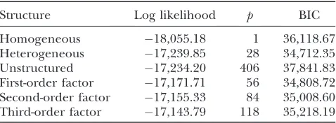
It is called factor analytic structure because this structure has been used in factor analysis. This factor analytic structure was derived on the basis of the fol-TABLE 1
BIC scores of the six variance–covariance structures for the barley data analysis
Structure Log likelihood p BIC
Homogeneous 18,055.18 1 36,118.67 Heterogeneous 17,239.85 28 34,712.35 Unstructured 17,234.20 406 37,841.83 First-order factor 17,171.71 56 34,808.72 Second-order factor 17,155.33 84 35,008.60 Third-order factor 17,143.79 118 35,218.19
The number of parameters is denoted byp.
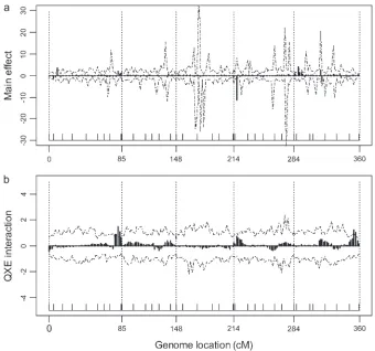
Figure1.—The estimated main and
lowing latent variable linear model for the residual errors,
jj ¼Buj1ej; ð29Þ
whereujis anr31 latent factor (r,m) with a
pðujÞ ¼Nðujj0;IrÞ ð30Þ
distribution, B is anm3rmatrix called factor loading, andejNð0;DÞis a vector of independent errors and D¼diag½d1d2 . . .dm is a diagonal matrix for the independent error variances.
Under the factor analytic structure, the MCMC algo-rithm requires sampling B and uj for j¼1,. . .,n, in addition to other parameters. We now describe the prior and posterior of these new variables. The prior forujis standardized multivariate normal given in Equation 30. The fully conditional posterior distribution remains multivariate normal,
pðujj . . .Þ ¼Nðujjmj;SjÞ; ð31Þ
where
mj¼ Ir1ðBTD1BÞ1
1
BTD1 yjb Xq
k¼1 Zjkgk
!
ð32Þ
and
Sj¼ Ir1ðBTD1BÞ1
1:
ð33Þ
The factor loadings are represented by anm3rmatrix B. Let Bl¼ ½Bl1 . . .BlmT be the lth column of matrix
Bforl¼1,. . .,r. We now rewrite Equation 29 as
jj¼ Xr
l¼1
Blujl1ej: ð34Þ
Givenuj and knowing that
jj¼yjb Xq
k¼1
Zjkgk; ð35Þ
Equation 34 is a typical multivariate regression problem. The fully conditional posterior distribution of Bl is multivariate normal,
pðBlj . . .Þ ¼NðBljml;SlÞ; ð36Þ
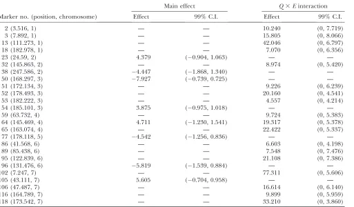
where TABLE 2
Estimated main andQ3Einteraction effects and their 99% confidence intervals of the null distributions for the barley yield data
Marker no. (position, chromosome)
Main effect Q3Einteraction
Effect 99% C.I. Effect 99% C.I.
2 (3.516, 1) — — 10.240 (0, 7.719)
3 (7.892, 1) — — 15.805 (0, 8.066)
13 (111.273, 1) — — 42.046 (0, 6.797)
18 (182.978, 1) — — 7.070 (0, 6.356)
23 (24.59, 2) 4.379 (0.904, 1.063) — —
32 (145.863, 2) — — 8.974 (0, 5.420)
38 (247.586, 2) 4.447 (1.868, 1.340) — —
50 (168.297, 3) 7.927 (0.739, 0.725) — —
51 (172.134, 3) — — 9.226 (0, 6.239)
52 (178.493, 3) — — 20.160 (0, 4.541)
53 (182.222, 3) — — 4.557 (0, 4.214)
54 (185.101, 3) 3.875 (0.975, 1.018) — —
59 (63.732, 4) — — 9.724 (0, 5.383)
64 (145.469, 4) 4.711 (1.230, 1.541) 19.317 (0, 5.378)
65 (163.074, 4) — — 22.422 (0, 5.337)
77 (178.118, 5) 4.542 (1.256, 0.836) — —
86 (41.568, 6) — — 6.603 (0, 4.198)
89 (85.438, 6) — — 7.548 (0, 7.476)
95 (122.839, 6) — — 21.108 (0, 7.386)
96 (131.476, 6) 5.819 (1.539, 0.884) — —
102 (7.247, 7) — — 77.311 (0, 5.606)
105 (43.111, 7) 5.605 (0.704, 0.958) — —
106 (47.487, 7) — — 16.614 (0, 6.140)
116 (164.789, 7) — — 9.899 (0, 5.959)
118 (173.542, 7) — — 33.210 (0, 3.860)
ml¼ X
n
j¼1 u2jlD1 " #1
Xn
j¼1
ujlD1ðjj Xr
l96¼l Bl9ujl9Þ
" #
¼ X
n
j¼1 u2jl " #1
Xn
j¼1
ujlðjj Xr
l96¼l Bl9ujl9Þ
" #
ð37Þ
and
Sl ¼ X
n
j¼1 u2jlD1 " #1
¼ X
n
j¼1 u2jl " #1
D: ð38Þ
Having provided the fully conditional posterior dis-tribution for every variable, we are now ready to conduct the Gibbs sampler to infer the empirical posterior dis-tribution for each variable.
APPLICATIONS
Barley data analysis: We used barley data obtained from the North American Barley Genome Mapping Pro-ject (Tinkeret al.1996) to demonstrate the application of
the new method. In the barley QTL mapping project, there were 127 mapped markers covering 1500 cM of the barley genome. Seven traits were investigated in the project. In this study, we used the yield trait analysis for the demonstration. The doubled haploid (DH) popula-tion was initiated from the cross between Harrington and
TR306. The DH population consisted of 145 lines, each grown in 28 different environments. The data set was updated after it was first published in 1996, but the difference between the original and the updated data was minor so that we could still compare the current result with that from the original study.
We used six different covariance structures to ana-lyze the data, which were (1) the homogeneous (con-stant) variance Q¼I28s2, (2) the heterogeneous
variancesQ¼D, (3) unstructured matrix Q(positive definite), (4) the first-order factor analytic structure
Q¼B2831BT113281D, (5) the second-order factor
ana-lytic structureQ¼B2832BT23281D, and (6) the
third-order factor analytic structure Q¼B2833BT33281D.
The length of the Markov chain consisted of 200,000 sweeps. The first 100,000 sweeps were deleted as burn-in and thereafter the chaburn-in was thburn-inned by keepburn-ing 1 observation in every 100 sweeps, producing 1000 obser-vations in the collected posterior sample for post-MCMC analysis.
To test the significance of the QTL effects, we con-ducted a permutation test to generate the null distribu-tion of each main effect and each Q 3 E interaction effect. In the permutation analysis, we repeated the MCMC sampling method as described before but re-shuffled the phenotypic values. The permutation anal-ysis was proposed by Cheand Xu(2010), who called it
permutation inside the Markov chain. In the permuta-tion analysis, the length of the Markov chain was 200,000
Figure2.—Estimated main andQ3E
sweeps. The first 100,000 sweeps were deleted as burn-in and the chain thinning rate was 1/25. The posterior sample contained 4000 observations. From the null distribution, we drew a confidence interval for each estimated effect. An effect was claimed to be significant if the estimated value fell outside of the 99% confidence interval of the null distribution.
Among the six covariance structures, the second structureQ¼D(a diagonal matrix) detected the maxi-mum number of QTL (main and Q 3 E interaction effects). Although more QTL does not mean better, it is hard to use cross-validation to evaluate different structures under the MCMC implemented Bayesian analysis. Bayes factors are often used to evaluate dif-ferent models. However, the complexity of our pro-posed model makes the calculation of the Bayes factors difficult. Therefore, we used the Bayesian information criteria (BIC) to evaluate the performance of the six different models. The BIC score was calculated using
BIC¼ 2 logðLÞ1plogðnÞ; ð39Þ
where L is the likelihood function evaluated at the estimated parameters,pis the number of parameters, andnis the sample size. The Bayesian estimates of the parameters inLare the posterior means ofb,g, andQ. The BIC scores are shown in Table 1, which indicates that the second (heterogeneous residual variance) model performed better than all other models. The
first-order factor analytic model was the second best model with a BIC score slightly larger than that of the best model. The result of the best model is depicted in Figure 1, where the posterior means of the main effects and the Q 3 E interaction effects are plotted against the genome locations of the markers. Figure 1 also gives the 99% confidence intervals for the main and Q3 E interaction effects. Eight markers showed significant main effects and 18 markers showed significantQ3 E interaction. The 18 interacting markers were distributed across all seven chromosomes of the entire genome. Only 1 marker had both the main and theQ3Einteraction effects. Each of the other markers had either a main effect or a Q 3 E interaction effect but not both. The estimated main and Q 3 E interaction effects for the markers are given in Table 2.
We also performed an individual marker analysis to compare the result with that of the Bayesian analysis. For the individual marker analysis, QTL mapping was conducted separately for each environment. The aver-age estimated effect for each marker across the 28 environments represented the main effect while the variance of the estimated effects across the environ-ments represented the Q 3 E interaction effect. The estimated main and Q 3 E interaction effects of the single-marker analysis are shown in Figure 2. We can see that Figure 2 is quite similar to Figure 1 in the Bayesian analysis. The main difference between the two figures is the different sharpness of the marker effects. The
Figure3.—Estimated main andQ3E
Bayesian analysis generated very clean (sharp) signals of the plots.
Arabidopsis data analysis: The barley data contain many environments, which is hard to find in most studies. So we also applied our model to recombinant inbred line data of Arabidopsis (Loudet et al. 2002),
where two parents initiating the line cross were Bay-0 and Shahdara, with Bay-0 as the female parent. Flower-ing time was recorded for each line in two environ-ments: long day (16-hr photoperiod) and short day (8-hr photoperiod). The population contained 420 lines. A total of 38 microsatellite markers were used for QTL mapping. We inserted a pseudomarker in every 2 cM of the genome and had a total of 200 markers (38 true markers plus 162 pseudomarkers) in our analysis.
The variance of Q 3 E interaction s2
k may not be estimated accurately due to small environments. So in small environments the variance would then simply serve as a tool to shrink the environment-specific QTL effects. The bias ofs2
k would lead to biased estimation of main effect as well. Although the MCMC algorithm remains the same as before, we need to revise our post-MCMC procedure. We use vectorgkto estimateQ3E interaction effects of the kth marker. The differences between vector gk and its mean represent Q 3 E interaction effects. In the two-environments case, we can just use the differences between the two compo-nents of gk as the Q 3 E interaction effects because vector gk is a 2 3 1 vector. Since there are only two environments, we did not use the factor analytic model Figure4.—The average main effects across 20 replicated simulation experiments for the entire genome in the first simulation
to analyze the data. The BIC scores for the three models (homogeneous, heterogeneous, and unstructured co-variance matrices) are 3798.49, 3775.64, and 3645.55. Figure 3 shows the main andQ3Einteraction effects of the Arabidopsis data under the unstructured co-variance model. The 95% confidence intervals for the main andQ3Einteraction effects are also given. Four markers showed significant main effects and six markers showed significantQ3Einteraction effects.
Simulation study: The barley data analysis did not show the advantage of fitting appropriate covariance structures over the simple diagonal covariance matrix because the 28 different environments did not seem to be correlated. Therefore, we conducted two simulation
experiments (simulations 1 and 2) in this section to demonstrate the importance of covariance structure to the Bayesian analysis ofQ3Einteraction. We also did a two-environment simulation (simulation 3) to demon-strate the fitness of our model for small environments.
In simulation 1, we used the real marker information from the North American Barley Genome Mapping Project (Tinkeret al.1996) to simulate the genome. We
simulated 127 markers from seven chromosomes with marker distances exactly the same as the real data. We simulated 145 DH lines in 28 environments. The in-terceptbwas given values ranging from 200 to 605 for the 28 different environments. We assumed that 10 of the 127 markers had main effects and also Q 3 E Figure5.—(a–f) The averageQ3Einteraction effects across 20 replicated simulation experiments for the entire genome in the
interaction effects in the 28 environments. In the simulation experiment, we chose the factor analytic covariance structureQ¼BBT1DwithBdefined as a 2833 matrix, indicating that correlations had occurred between different environments. The true values ofb, the QTL effects, theBmatrix, and theDmatrix are given in Tables 4 and 5. The simulated data were analyzed using the six different covariance structures described earlier in the barley data analysis. We expected that the first three structures (homogeneous variance, hetero-geneous variance, and unstructured matrices) would perform poorly but the last three structures (first-order, second-order, and third-order factor analytic structures) would perform better, especially the third-order factor analytic structure.
In the MCMC-implemented Bayesian analysis, the length of the Markov chain was 50,000 sweeps. The first 25,000 sweeps (burn-in period) were deleted. The chain thinning rate was 1 in 50. The empirical posterior sample contained 500 observations for the post-MCMC analysis. The MCMC experiment with the same simu-lated data was repeated a few times to make sure that the
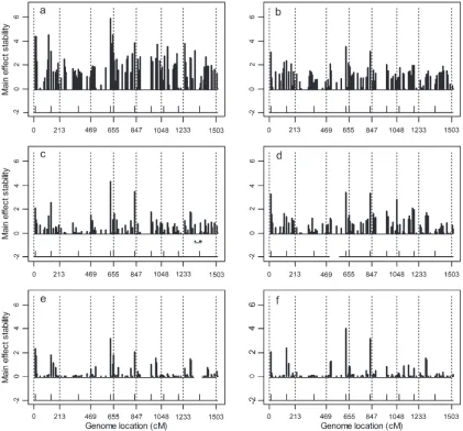
chain had converged to the stationary distribution. The results of the simulation studies are depicted in Figure 4 for the average main effects of 20 replicates and in Figure 5 for the averageQ3Einteraction effects of 20 replicates. These two figures show that the estimated QTL effects agreed well with the true effects. Figures 4 and 5 also show that the first four covariance structures (ho-mogeneous residual, heterogeneous residual, unstruc-tured covariance, and first-order factor analytic structure) have some notable background noise, indicating some false positives had occurred. However, the last two factor analytic structures have very little background noise. From the two figures, the background noise of the first four covariance structures may not be very clear. So we calculated standard deviations of each marker’s main effect among the 20 replicates and plotted them in Figure 6, from which we can see the difference among the six models. The performance of the last two factor analytic models is very stable for the majority of the markers without main effects. While the first four structures, especially the first two, cannot achieve such a nice performance, which means that among the 20 replicates TABLE 3
Average BIC score for six different variance–covariance structures in the simulation study
Covariance structure Log likelihood p BIC
Homogeneous 18,096.83 1 36,201.97 Heterogeneous 17,564.80 28 35,362.26 Unstructured 16,815.18 406 37,003.79 First-order factor 17,176.53 56 34,818.36 Second-order factor 16,887.74 84 34,473.44 Third-order factor 16,858.56 118 34,647.73
The number of parameters is denoted byp.
TABLE 4
True and estimated QTL main effects andQ3Einteraction
effects from 20 replicated simulation experiments under the second-order factor analytic covariance structure
Marker no. (position, chromosome)
Main effect Q3E
True Estimated True Estimated
1 (0, 1) 5 1.14 36 41.33
14 (127.208, 1) 7 6.51 0.25 0.20 32 (145.863, 2) 1 0.01 16 19.76 48 (153.931, 3) 10 8.08 4 2.38 52 (178.493, 3) 4 0.75 25 22.45 65 (163.074, 4) 8 8.14 49 45.03 71 (109.389, 5) 15 15.52 9 7.66 84 (10.533, 6) 1 0.00 1 0.25 96 (131.476, 6) 0 0.00 64 65.64 110 (122.584, 7) 3 0.01 100 123.19
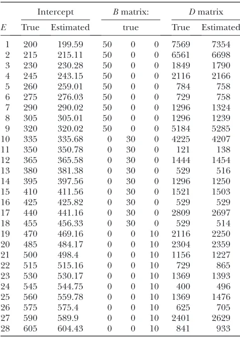
TABLE 5
The true and estimated intercepts, theBandDmatrices used in simulation 1
E
Intercept Bmatrix: Dmatrix
True Estimated true True Estimated
1 200 199.59 50 0 0 7569 7354 2 215 215.11 50 0 0 6561 6698 3 230 230.28 50 0 0 1849 1790 4 245 243.15 50 0 0 2116 2166 5 260 259.01 50 0 0 784 758 6 275 276.03 50 0 0 729 758 7 290 290.02 50 0 0 1296 1324 8 305 305.01 50 0 0 1296 1239 9 320 320.02 50 0 0 5184 5285 10 335 335.68 0 30 0 4225 4207 11 350 350.78 0 30 0 121 138 12 365 365.58 0 30 0 1444 1454 13 380 381.38 0 30 0 529 516 14 395 397.56 0 30 0 1296 1250 15 410 411.56 0 30 0 1521 1503 16 425 425.82 0 30 0 529 529 17 440 441.16 0 30 0 2809 2697 18 455 456.33 0 30 0 529 514 19 470 469.16 0 0 10 2116 2250 20 485 484.17 0 0 10 2304 2359 21 500 498.4 0 0 10 1156 1227 22 515 515.16 0 0 10 729 865 23 530 530.17 0 0 10 1369 1393 24 545 544.75 0 0 10 400 496 25 560 559.78 0 0 10 1369 1476 26 575 575.4 0 0 10 625 705 27 590 589.9 0 0 10 2401 2629 28 605 604.43 0 0 10 841 933
these models generated some false main effects. Table 3 shows the average BIC scores for the six different covariance structures. We see that the factor analytic structure outperformed the other three models. This is consistent with our expectation. The lowest BIC occurred in the second-order factor analytic structure. However, the third-order factor analytic structure (the true model) was just slightly higher in value than the second-order structure. The log-likelihood value of the third-order factor was higher than that of the second-order factor. Table 4 gives the average estimated main and Q 3 E interaction effects obtained from the 20 replicates based on the second-order factor analytic model. When we compared the estimated main effects and the true effects, we noted that large main effects were estimated quite accurately but small effects were shrunken to zero. The Q3Einteraction effects were always detectable regard-less of the sizes of the effects. Table 5 gives the true intercepts and the residual error variances (theDmatrix)
along with their estimated values. The trueBmatrix is also given in Table 5. The estimated B was not given here because the columns ofBare independent and thus are exchangeable. This does not affect the estimate of the covariance structure. We checked the average estimated variance–covariance matrix and did observe three sepa-rate environment groups.
Although the stability test and BIC scores showed the advantage of the factor analytic model, the differences of marker main effects for the six models are not very obvious in Figure 4. So we performed the second sim-ulation experiment (simsim-ulation 2) to further demon-strate the advantage of the factor analytic model. We focused mainly on comparison of heterogeneous di-agonal structure and three factor analytic models. In this simulation, 100 DH lines in eight environments were generated with 30 markers. The distance between two nearby markers was 30 cM. The intercept b was given values ranging from 200 to 305 for the eight Figure6.—(a–f) The standard deviations (stabilities) of estimated main effects across 20 replicated simulation experiments for
environments. We assumed that 3 of the 30 markers had main effects and alsoQ 3 E interaction effects in the eight environments. We also chose the factor analytic covariance structureQ¼BBT1DwithBdefined as an 832 matrix. The first column ofBhad values of 20, 10, 10, 5, 0, 0, 0, 0. The second column had values of 0, 0, 0, 0, 15, 15, 10, 2. MatrixDwas an identity matrix. Figure 7 shows the estimated main effects of the four models. We can clearly see many false positive main effects in the heterogeneous diagonal structure. The BIC scores for the four models are 4264, 3362, 2495, and 2558, which also are in favor of the factor analytic models.
In simulation 3, we also generated 100 DH lines using the same marker information given by simulation 2, but this time we simulated only two environments. The intercepts were 200 and 215 for the two environments. The factor analytic covariance structure was used withB defined as a 232 matrix. The first column of B had values of 1 and 2. The second column had values of 2 and 1. MatrixDwas an identity matrix. The MCMC and post-MCMC analyses of these data used the same setup as Arabidopsis data analysis. Figure 8 gives the compar-ison of the true and the estimated main and Q 3 E interaction effects. From Figure 8, the true and the estimated marker effects are very close to each other for all three models. The promising results also demon-strate that our proposed method is a good choice to handle data with small environments.
DISCUSSION
The importance of this study is reflected by two major contributions toQ3 Estudy, the multiple-QTL
model and the factor analytic covariance structure. The multiple-QTL model for Q3 E is an extension of the Bayesian shrinkage analysis for mapping QTL in a single environment (Xu2003). The factor analytic covariance
structure is available in the literature but has never been applied to QTL mapping. Other covariance structures may be considered in future studies, e.g., the autore-gressive model of order 1 [AR(1)] and compound symmetry (CS) covariance structures. These alternative structures can be used to fit models when the environ-ments represent temporal or spatial variation. The 28 environments in the barley experiments represent 28 different locations (spatial variation). However, the information about the location was not available to us. We believe that the factor analytic structure is robust and can be fit to a wide variety of covariance structures, ranging from the simplest diagonal matrix to the most complicated unstructured matrix, by choosing different orders of the factors. This has been demonstrated by the similarity of the diagonal matrix and the first-order factor analytic model in our data analyses. The factor analytic model is also easy to fit under the general linear model framework. Both the factor loadings and the factors themselves have normal posterior distributions and can be sampled using the Gibbs sampler approach. The most significant contribution of this study was to use the variance of QTL effects across environments to measure the size of theQ3Einteraction for a particular QTL. This has significantly simplified theQ3Estudy. If the number of environments were small, however, the variance would not be accurately estimated. In this case, one should use some kind of linear contrast of the environment-specific effects as a measure of theQ3 E
Figure7.—The marker main effects
interaction. Arabidopsis data and simulation 3 are two examples of such a treatment. The variance would then simply serve as a tool to shrink the environment-specific QTL effects. The MCMC sampling procedure remains the same, but the post-MCMC analysis needs to be modified. The method developed in the current study applies only to plants where the same genotype can be replicated in multiple environments. In animals where the same genotype cannot be replicated (except identical twins), some modification is required. For example, if an F2family
is raised in three environments, each animal may have a different genotype from other animals. This argument also applies to QTL-by-sex interaction, where the same individual cannot be split into male and female. The modification is not trivial and thus deserves further study.
Although the environment-specific QTL effects, de-noted by vectorgkfor thekth marker, are used only to draw the posterior distributions for the main andQ3E interaction effects, they may be interesting parameters in their own rights. The posterior mean of eachgkcan be used to predict the molecular breeding value of each line in a particular environment. This information may facilitate marker-assisted selection (using a few markers) or genome selection (using all markers of the entire genome). Genome selection has been an important strategy for animal (Meuwissenet al.2001) and plant
breeding (Xu2003).
The Bayesian method presented here applies only to multiple-marker analysis;i.e., each marker is treated as a putative QTL. If the markers are not evenly placed in the Figure8.—The marker main effects andQ3Einteraction effects in the third simulation experiment. (a and b) Homogeneous
genome, one may insert some pseudomarkers in regions not well covered by markers. In the regions with saturated markers, one may use only a few selected markers to avoid a potential multicollinearity problem. With the current molecular technology, genomes of most species of agricultural importance may be satu-rated very soon with high-density markers. Pseudo-marker insertion will no longer be necessary, but marker selection will become important. One strategy for marker selection is to include one marker in every dcM for the Bayesian model. The optimal strategy may be the moving interval approach proposed by Wanget al.
(2005), in which a fixed number of putative QTL were included in the model for each chromosome and the position of the putative QTL can move ( jump) among a few neighboring markers. This approach may be adop-ted in the second stage of mapping,i.e., fine mapping after the important QTL regions have been identified.
One drawback of the MCMC-implemented Bayesian method is the slow computation process due to the large number of environments and the high dimensionality of the model. A quick method may be the posterior mode estimation in which only the conditional poste-rior modes are presented as the Bayesian estimates for the parameters of interest. Although the estimates are no longer Bayesian estimates, the results may be comparable. This quick posterior mode estimation may provide preliminary results to be used for further analysis using the fully Bayesian analysis.
Finally, the entire data analyses were conducted using a program developed in R. Interested readers may visit our website (www.statgen.ucr.edu) to download the program and the sample data to test the method and analyze their own data.
This project was supported by the National Plant Genome Initiative of the U.S. Department of Agriculture Cooperative State Research, Education, and Extension Service grant 2007-02784 (to S.X.).
LITERATURE CITED
Beavis, W. D., and P. Keim, 1996 Identification of quantitative trait loci that are affected by environment, pp. 123–150 in Genotype-by-Environment Interaction, edited by M. S. Kangand H. G. Gauch. CRC Press, Boca Raton, FL.
Boer, M. P., D. Wright, L. Feng, D. W. Podlich, L. Luoet al., 2007 A mixed-model quantitative trait loci (QTL) analysis for multiple-environment trial data using environmental covariables for QTL-by-environment interactions, with an example in maize. Genetics177:1801–1813.
Che, X. and S. Xu, 2010 Significance test and genome selection in Bayesian shrinkage analysis. Int. J. Plant Genomics doi:10.1155/ 2010/893206
Jansen, R. C., 1993 Interval mapping of multiple quantitative trait loci. Genetics135:205–211.
Jansen, R. C., J. W. Ooijen, P. Stam, C. Lister and C. Dean, 1995 Genotype-by-environment interaction in genetic map-ping of multiple quantitative trait loci. Theor. Appl. Genet.
91:33–37.
Jiang, C., and Z. B. Zeng, 1995 Multiple trait analysis of genetic mapping for quantitative trait loci. Genetics140:1111–1127. Lander, E. S., and D. Botstein, 1989 Mapping Mendelian factors
underlying quantitative traits using RFLP linkage maps. Genetics
121:185–199.
Loudet, O., S. Chaillou, C. Camilleri, D. Bouchez and F. Daniel-Vedele, 2002 Bay-03Shahdara recombinant inbred line population: a powerful tool for the genetic dissection of com-plex traits in Arabidopsis. Theor. Appl. Genet.104:1173–1184. Meuwissen, T. H., B. J. Hayesand M. E. Goddard, 2001 Prediction
of total genetic value using genome-wide dense marker maps. Genetics157:1819–1829.
Paterson, A. H., S. Damon, J. D. Hewitt, D. Zamir, H. D. Rabinowitch
et al., 1991 Mendelian factors underlying quantitative traits in tomato: comparison across species, generations, and environ-ments. Genetics127:181–197.
Piepho, H. P., 2000 A mixed-model approach to mapping quantita-tive trait loci in barley on the basis of multiple environment data. Genetics156:2043–2050.
Romagosa, I., S. E. Ullrich, F. Hanand P. M. Hayes, 1996 Use of the additive main effects and multiplicative interaction model in QTL mapping for adaptation in barley. Theor. Appl. Genet.93:
30–37.
Stuber, C. W., S. E. Lincoln, D. W. Wolff, T. Helentjarisand E. S. Lander, 1992 Identification of genetic factors contributing to heterosis in a hybrid from two elite maize inbred lines using mo-lecular markers. Genetics132:823–839.
terBraak, C. J. F., M. P. Boerand M. Bink, 2005 Extending Xu’s Bayesian model for estimating polygenic effects using markers of the entire genome. Genetics170:1435–1438.
Tinker, N. A., D. E. Mather, B. G. Rossnagel, K. J. Kasha, A. Kleinhofset al., 1996 Regions of the genome that affect ag-ronomic performance in two-row barley. Crop Sci.36:1053–1062. Wang, H., Y. M. Zhang, X. Li, G. L. Masinde, S. Mohan et al., 2005 Bayesian shrinkage estimation of quantitative trait loci parameters. Genetics170:465–480.
Xu, S., 2003 Estimating polygenic effects using markers of the entire genome. Genetics163:789–801.
Zeng, Z. B., 1994 Precision mapping of quantitative trait loci. Genet-ics136:1457–1468.