Non-Linear Gradient Descent Algorithm for Smart Antennas

(1)

ISSN(Online): 2320-9801

ISSN (Print) : 2320-9798

I

nternational

J

ournal of

I

nnovative

R

esearch in

C

omputer

and

C

ommunication

E

ngineering

(An ISO 3297: 2007 Certified Organization)

Vol. 3, Issue 9, September 2015

Non-Linear Gradient Descent Algorithm for

Smart Antennas

P Pyad Koteswara Rao, Dr. Y. Ramakrishna, Dr. P.V Subbaiah

M. Tech Student, Dept. of E.C.E, PVPSIT, Vijayawada, Andhra Pradesh, India

Associate Professor, Dept. of E.C.E, PVPSIT, Vijayawada, Andhra Pradesh, India

Professor, Dept. of E.C.E, VRSEC, Vijayawada, Andhra Pradesh, India

ABSTRACT: A Nonlinear Gradient Descent algorithm (NGD) is an iterative method that is given an initial point and

follows the negative of the gradient in order to move the point towards a critical point, which is hopefully the desired local minimum. Nonlinear gradient descent is a popular algorithm for very large scale optimization problems, because it is easy to implement and can handle black box functions [1]. In Smart Antennas (SA) both Half Power Beam Width (HPBW) and Side Lobe Level (SLL) are low values to get good performance. However to design smart antennas with minimum side lobe level, and HPBW, Nonlinear gradient descent algorithm gives the good performance on HPBW and SLL. This NGD algorithm is used for adaptive array smart antennas, because these arrays allows the antenna to steers the beam pattern in order to enhance the reception of a desired signal, while simultaneously suppressing interfering signals through complex weight selection.

KEYWORDS: NGD algorithm, HPBW, SLL, step size parameter, smart antenna

.

I. INTRODUCTION

(2)

ISSN(Online): 2320-9801

ISSN (Print) : 2320-9798

I

nternational

J

ournal of

I

nnovative

R

esearch in

C

omputer

and

C

ommunication

E

ngineering

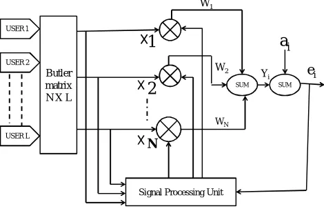
1

2

N Butler

matrix N X L

USER 1

USER 2

USER L

Signal Processing Unit

SUM SUM

W1

W2

WN

Yi ei

a

_i

Figure 1. Basic smart antenna

Related work

Dai and Yuan proposed the nonlinear gradient descent method which generates a descent search direction at every iteration. In this paper, is proposed a nonlinear gradient descent method based on the study of Dai and Yuan and show that this method always produces a descent search direction. The numerical results show that this method is very efficient for given standard test problems [5]-[6].

II. PROPOSED ALGORITHM

The equations that describe the nonlinear gradient descent algorithm for a complex-valued dynamical perceptron, with a single output neuron are given by

e(k) =d(k) – y(k), y(k) =Φ(net(k)) (1)

where e(k) is the instantaneous output error of the filter at time instant k, y(k) is the output from the nonlinear activation function, d(k) is the desired output, ɸ(net(k) is some holomorphic function that is bounded everywhere in the complex domain [7].

net(k) =∑ x (k) (k) =X (k) w(k) (2) Where x(k) denotes the input such that

(k) =x (k – n + 1), n = 1………,N.

W(k) is the weight vector and is equals to [w (k),……,w (k)] rise to the power T, and N is the number of array elements used. For simplicity we state that,

Φ(net(k)) = Φ (net(k)) + j Φ (net(k)) = u(k) + jv(k) (3) Where the superscripts (. ) and (. ) respectively, denotes the real and imaginary parts of a complex quantity, and j =√−1. It can be split up the error term in equation (1), into its real and imaginary parts as

e (k) = d ( ) – u(k), e(k) = d ( ) – v(k) (4) E(k) = |e(k)|2

= [e (k)e∗_{(k)] = [(}_e ₎2

(k) + (e)2(k)] (5) Where E(k) is the conventional cost function and (. )∗_{denotes the complex conjugate. The weight adaptation in the} NGD algorithm is therefore given by equation (3)

w (k+1) = w (k) + ∆w (k), n = 1, 2,…..,N (6) ∆w (k) = –η∇ [E(k)] ( )

= η e(k)(Φ/_[net(k)])∗_x∗_(k) ₍₇₎ Where η is the learning rate. The NGD algorithm can be written in the compact form as

(3)

ISSN(Online): 2320-9801

ISSN (Print) : 2320-9798

I

nternational

J

ournal of

I

nnovative

R

esearch in

C

omputer

and

C

ommunication

E

ngineering

Learning rate is a decreasing function of time [8]. Two forms that are commonly used are a linear function of time and a function that is inversely proportional to the time t.

III.SIMULATION RESULTS

The simulations are carried out with an input signal x (k) = cos(2wt) at frequency of 1kHz along with a random

noise. When the values of N and μ (step size parameter) are varied, one can generate main lobe in required direction

with low SLL and HPBW [9]-[10]. At N=8, Signal to Noise Ratio (SNR) =45, when the μ value is increased it is

observed that HPBW is also increasing simultaneously reducing SLL, as shown in table 1.

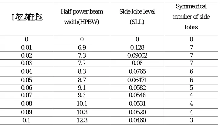
Table 1. Performance of HPBW and SLL by increasing μ values.

Step size(μ) Half power beam

width(HPBW)

Side lobe level

(SLL)

Symmetrical

number of side

lobes

0 0 0 0

0.01 6.9 0.128 7

0.02 7.3 0.09002 7

0.03 7.7 0.08 7

0.04 8.3 0.0765 6

0.05 8.7 0.06471 6

0.06 9.1 0.0582 5

0.07 9.3 0.0546 4

0.08 10.1 0.0531 4

0.09 10.3 0.0520 4

0.1 12.3 0.0460 3

In order to simulate the real time environment of smart antenna system, the noise component has been considered in addition to the input signal and the performance of the Nonlinear gradient descent algorithm have been analyzed with different values of N and constant step size (μ), as result in decreasing HPBW, SLL as shown in below

table 2.

Table 2. Performance of HPBW and SLL by increasing N values.

Number of array element (N)

Half power beam width

(HPBW) Side lobe level (SLL)

1 60 -

2 26.5 0.2577

3 17.5 0.2143

4 13.3 0.1792

5 10.8 0.1548

6 10.1 0.133

7 8.1 0.0999

8 7.3 0.09168

9 6.7 0.0842

(4)

ISSN(Online): 2320-9801

ISSN (Print) : 2320-9798

I

nternational

J

ournal of

I

nnovative

R

esearch in

C

omputer

and

C

ommunication

E

ngineering

IV.CHARACTERISTICSOFSMARTANTENNAWITHNGDALGORITHM

The characteristics of normalized array factor is plotted, for N=8, μ=0.02, by taken, angle (in degree) on x-axis, normalized array factor on y-axis, the corresponding results for HPBW and SLL are 7.3 and 0.08977 respectively, as shown in figure 2. For the above mentioned values of N and μ, the comparison of array output of NGD algorithm (shown in dotted line), with desired output (shown in thick line), by taken number of iterations on x-axis and normalized signal amplitude on y-axis, corresponding characteristics are as shown in figure 3.

Figure 2. Normalized Array factor generated with NGD algorithm. Figure 3 Comparison of array output of NGD algorithm, with desired output.

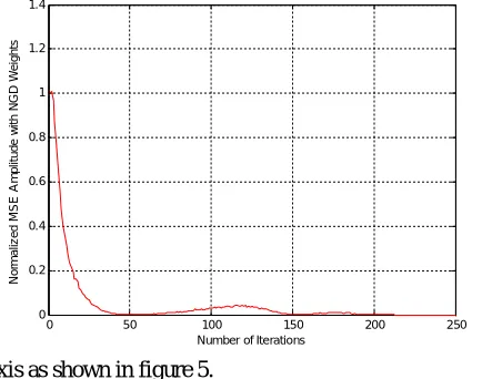
The Mean Square Error (MSE) of an estimator measures the average of the squares of the "errors", that is, the difference between the estimator and what is estimated. MSE is a risk function, corresponding to the expected value of the squared error loss or quadratic loss [11]. By taken number of iterations on x- axis, normalized MSE amplitude on y- axis, the corresponding characteristics as shown in figure 4. At different values of N, the characteristics of normalized array factor and it’s corresponding side lobe levels are plotted by taking angles on x- axis, normalized array factor on y-

axis as shown in figure 5.

Figure 4. Normalized mean square error generated with NGD algorithm. Figure 5. Normalized Array factor generated with NGD algorithm.

By taken number of iterations on x- axis, normalized MSE amplitude on y- axis, the corresponding characteristics at different values of N, as shown in figure 6. For the different values of N, the comparison of array output of NGD algorithm, with desired output, plotted by taken number of iterations on x-axis and normalized signal amplitude on y-axis, corresponding characteristics are as shown in figure 7.

0 50 100 150 200 250

-1 -0.8 -0.6 -0.4 -0.2 0 0.2 0.4 0.6 0.8 1

Number of Iterations

N o rm a liz e d S ig n a l A m p lit u d e

Comparison of Array output of NGD Algorithm with Desired output

Desired Signal NGD

-1000 -80 -60 -40 -20 0 20 40 60 80 100 0.1 0.2 0.3 0.4 0.5 0.6 0.7 0.8 0.9 1 Angle (Degrees) N o rm a liz e d A rr a y F a c to r

Array Factor with NGD Weights

0 50 100 150 200 250

0 0.2 0.4 0.6 0.8 1 1.2 1.4

N o rm a liz e d M S E A m p lit u d e w it h N G D W e ig h ts

-1000 -80 -60 -40 -20 0 20 40 60 80 100 0.1 0.2 0.3 0.4 0.5 0.6 0.7 0.8 0.9 1 Angle (degrees) N o rm a liz e d a rr a y f a c to r

Array factor with NGD weights

(5)

ISSN(Online): 2320-9801

ISSN (Print) : 2320-9798

I

nternational

J

ournal of

I

nnovative

R

esearch in

C

omputer

and

C

ommunication

E

ngineering

Figure 6. Normalized mean square error (MSE) generated with NGD algorithm. Figure 7. Comparison of array output of NGD with desired output.

V. COMPARISONOFWEIGHTEDANDUNWEIGHTEDOUTPUTS

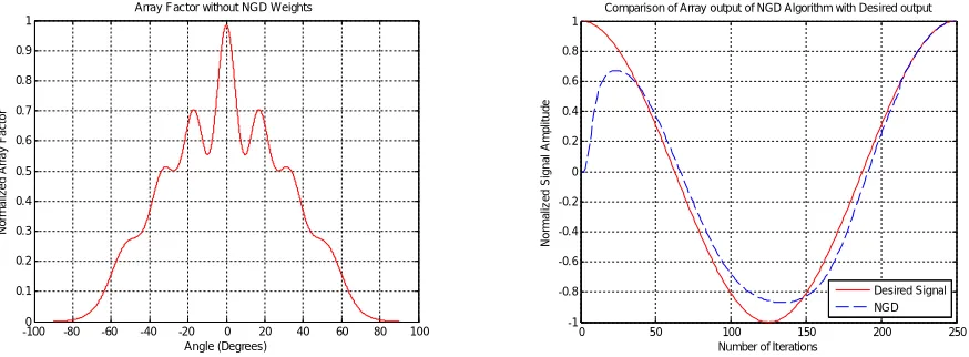
Number of array elements and step size are fixed at the values of, 8 and 0.02 respectively, the characteristics of normalized array factor obtained with un-weighted, as shown in figure 8. For the above mentioned values of N and

μ, the comparison of array output for un-weighted (shown in dotted line), with desired output (shown in thick line),

corresponding characteristics are as shown in figure 9.

Figure 8. Normalized Array factor generated without NGD algorithm. Figure 9. Comparison of array output of NGD algorithm, with desired output.

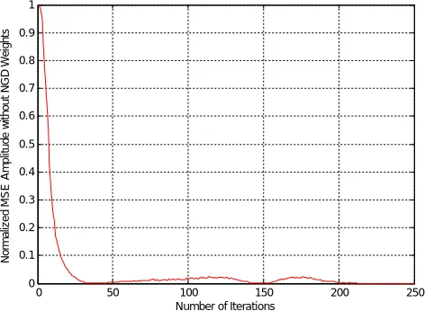
Normalized MSE amplitude for un-weighted can be plotted, By chosen number of iterations on x- axis, normalized MSE amplitude on y- axis, the corresponding characteristics as shown in figure 10.

0 50 100 150 200 250

-1 -0.8 -0.6 -0.4 -0.2 0 0.2 0.4 0.6 0.8 1

N o rm a li z e d S ig n a l A m p lit u d e

N=8 N=6 N=4 Desired signal

0 50 100 150 200 250

-1 -0.8 -0.6 -0.4 -0.2 0 0.2 0.4 0.6 0.8 1

N o rm a li z e d S ig n a l A m p li tu d e

Desired Signal NGD

0 50 100 150 200 250

0 0.1 0.2 0.3 0.4 0.5 0.6 0.7 0.8 0.9 1

N o rm a li z e d M S E A m p lit u d e w it h N G D W e ig h ts N=4 N=6 N=8

-1000 -80 -60 -40 -20 0 20 40 60 80 100 0.1 0.2 0.3 0.4 0.5 0.6 0.7 0.8 0.9 1 Angle (Degrees) N o rm a li z e d A rr a y F a c to r

(6)

ISSN(Online): 2320-9801

ISSN (Print) : 2320-9798

I

nternational

J

ournal of

I

nnovative

R

esearch in

C

omputer

and

C

ommunication

E

ngineering

Figure 10. Normalized mean square error generated for un-weighted.

VI.CONCLUSION AND FUTURE WORK

Nonlinear gradient decent algorithm is considered for adaptive beam forming of signals in smart antennas, with various parameters such as number of array elements, learning rate, step size of adaptive amplitude, have been considered under noiseless and noisy environments. From the analysis with NGD weights have better performance in the convergence of desired signal, in giving low HPBW and SLL in noiseless environment.

However un-weighted has no control over adaptation of HPBW and SLL. At the same time NGD weights has good control over adaptation of these two parameters with η and μ. By using NGD weights we designed a smart

antenna with minimum half power beam width and side lobe level.

REFERENCES

[1] Andrew I. Hanna and D. P. Mandic, "A complex-valued nonlinear neural adaptive filter with a gradient adaptive amplitude of the activation function”, Journal of Neural Networks, vol. 16, issue 2, pp. 155-159, 2003.

[2] D. P. Mandic, “NNGD algorithm for neural adaptive filters,” Electron.Lett., vol. 39, no. 6, pp. 845–846, 2000.

[3] Y. Ramakrishna, PESN Krishna Prasad, P.V. Subbaiah and B. Prabhakara Rao, “A Performance Analysis of CLMS and Augmented CLMS

Algorithms for Smart Antennas ", Proc. 4th International Workshop on Computer Networks and Communications, Coimbatore 2012, pp. 9-19, DOI: 10.5121/csit.2012.2402.

[4] Smart Antennas – Beam forming Tutorial”, www.altera.com

[5] Y. H. Dai and Y. Yuan, A Nonlinear Conjugate Gradient Method with Nice Global Convergence Properties, Research report ICM-95-038, Institute of Computational Mathematics and Scientific/Engineering Computing, Chinese Academy of Sciences, 1995.

[6] Y. H. Dai and Y. Yuan, Convergence properties of the conjugate descent method, Adv. Math. (China), 26 (1996), pp. 552–562

[7] D. P. Mandic and Vanessa Su Lee Goh, “Complex Valued Nonlinear Adaptive Filters – Noncircularity, Widely Linear and Neural Models”, John Wiley & Sons Ltd., 2009.

[8] A. I. Hanna, D. P. Mandic, and M. Razaz, “A normalized backpropagation learning algorithm for multilayer feed-forward neural adaptive filters,” in Proc. XI IEEE Workshop Neural Networks Signal Process., 2001, pp. 63–72.

[9] D. P. Mandic and J. A. Chambers, “Toward the optimal learning rate for backpropagation,” Neural Process. Lett., vol. 11, no. 1, pp. 1–5, 2000. [10] V. J. Mathews and Z. Xie, “Stocastic gradient adaptive filters with gradient adaptive stepsizes,”IEEE Trans. Signal Processing, vol. 41, pp.

2075–2087, June 1993.

[11] D. Mandic and J. Chambers, Recurrent Neural Networks for Prediction. New York: Wiley, 2001.

0 50 100 150 200 250

0 0.1 0.2 0.3 0.4 0.5 0.6 0.7 0.8 0.9 1

N

o

rm

a

liz

e

d

M

SE

Am

p

lit

u

d

e

w

it

h

o

u

t

N

G

D

W

e

ig

h

(7)

ISSN(Online): 2320-9801

ISSN (Print) : 2320-9798

I

nternational

J

ournal of

I

nnovative

R

esearch in

C

omputer

and

C

ommunication

E

ngineering

BIOGRAPHY

Mr. P. Koteswara Rao is pursuing M. Tech degree in Microwave and Communication Engineering at PVP Siddhartha Institute of Technology, Vijayawada, India. He had obtained B.Tech degree from the same institute in 2012.

Dr. Y. Ramakrishna is currently working as Associate Professor at PVP Siddhartha Institute of Technology, Vijayawada, India. He had obtained Ph.D. from JNTU Kakinada in the field of Smart Antennas for Mobile Communications. He received M.Tech Degree in Microwave Engineering from Acharya Nagarjuna University, India in 2005. He is a Member of ISTE, IETE. His Research interest includes Smart Antennas, Mobile Communications and Microwave Engineering.